DOI: 10.12928/TELKOMNIKA.v15i1.3892 448
Face Alignment using Modified Supervised Descent
Method
Mochammad Hosam, Helmie Arif Wibawa*, Aris Sugiharto
Informatics Department, Faculty of Science and Mathematics, Diponegoro University, Jl. Prof Sudharto, SH, Tembalang, Semarang, Central Java, Indonesia
*Corresponding author, e-mail: [email protected]
Abstract
Face alignment has been used on preprocess stage in computer vision’s problems. One of the best methods for face aligment is Supervised Descent Method (SDM). This method seeks the weight of non-linear features which is used for making the product and the feature resulting estimation on the changes of optimal distance of early landmark point towards the actual location of the landmark points (GTS). This article presented modifications of the SDM on the generation of some early forms as a sample on the training stage and an early form on the test stage. In addition, the pyramid image was used as the image for feature extraction process used in the training phase on linear regression. 1€ filter was used to stabilize the movement of estimated landmark points. It was found that the accuracy of the method in BioID dataset with 1000 training images in RMSE is approximately 0.882.
Keywords: supervised descent method, 1€ Filter, face alignment, computer vision
Copyright © 2017 Universitas Ahmad Dahlan. All rights reserved.
1. Introduction
There are other terms for alignment of facial landmarks, namely face alignment, facial landmark localization, facial feature detection, etc. Basically, face alignment is a problem of image registration. Generally, the process of face alignment tries to deform models, templates or facial features that correspond to the facial image [1]. The face shape in the context of face alignment is a set of the facial landmark point. The landmark point which is resulted from face alignment process representing facial features function as the main information of facial geometry.
Face alignment is pre-stage process in various computer visions of face-related problems [2]. Face alignment produces facial features which are used in the next process. Therefore, the higher the level of accuracy of face alignment method, the better the feature swhich are resulted, and the higher the success rate of the system [3]. Several issues require face alignment is 3D facial modeling, estimation pose, expression analysis, face recognition, facial animation, gaze tracking, etc [2, 4]. Real-time face alignment of the video is very important for many applications such as analysis of facial expression, monitors the level of driver's weariness, etc [2]. In addition, face alignment is included into the field of computer vision problems and as described in [5], computer visionis an important tool in the robotic system.
One of the best methods in resolving face alignment is Supervised Descent Method (SDM) [6]. This method minimizes the errors resulted from the weight product with a non-linear feature extraction with the obtained feature values to reach the value change of the optimum distance between face shape actual initialization with the real face shape. SDM uses regression as one of the steps in the training process. The step of generating initial sample face is an essential step affecting the results of the regression.
Further, variations in facial features caused by the shape, pose, lighting, expression, and image resolution make face alignment become a challenging problem [4]. SDM works well on static images. On the other hand, video has a fairly high noise and dynamic facial movement. The movement of the point of landmark results of face alignment between its frames tend to be unstable, rough and unnatural. This results 2 effects i.e. jitter and lag. As the first often occur in slow facial movements, the latter often occur in rapid facial movements. One way to overcome these effects, the movement of the face can be seen as a sequence of an event. These events
value, so that the lag effect can be reduced. Conversely when the face moves slowly, 1€ will
reduce the value of the cutoff frequency so that the effect of jitter is reduced.
Regarding to the step of initial sample face this article presents a modified method in that step. Besides, the pyramid image was used as the base image for extracting non-linear features and HOG was applied as a non-linear feature extraction function. Futhermore, this
article describes the use of € 1 filter as a filter in the process of face alignment using SDM on
video. It succesfully increase the stability of the movement of facial shape, improving smoothness and can cope with noise, as well as be able to parse the effects of jitter and lag in the movement of the point of landmark results of face alignment between frames.
2. Research Method
SDM refers to [6] and its application is divided into three stages:
1. Pre-Training. It is a stage for image processing in the dataset to be used at training stage.
2. Training. It isa feature of training stage (in this case, it uses the HOG descriptor) to gain weight for fitting process,
3. Fitting,. It is a stageto detect the position of facial landmarks in the test image using models or the weight resulted from the training.
2.1. Pre-training
This phase consists of several important processes, namely: 1. Extract the entire area of the face on the training data.
This process begins by detecting the face at the whole data. As discussed in [7], basically, the face detection is a separation process of facial images and background. It means also determining the specific location, size and quantity or the amount of face if there are one or more pictures of faces or there is even no image at all.
The next step is to calculate the average of the detection results. Then, the whole pictures in the dataset are transformed. This makes the size of the detection results at each of the data close to the average results of detection. The next step is to extract the image on the area of the detection results at the whole image in the dataset. The final result of this process is an image of face area with almost same size. The average results of the detection are also used as a reference image size at the fitting stage. Each image which is processed on the stage has to be scaled so that the size of the detection results close to the average size. In addition, the calculation accuracy also happens on the average size ofthe face.
The calculation of the average GT Scan be described as follows: for example, and are the position of the landmark tot on x and y coordinates sequentially, is a matrix of one-dimensional ground truth face shape of data ion a data set with elements of and z is a number ofland mark points on the shape ofthe face, setaris theamountof training data so thattheshape ofthe average face ̅ can be obtained by equation(1).
̅ ∑ (1)
2. Transforming the GTS average approaching GTS at each training
This process is trying to obtain a number of transformation matrixes which is used as training data in the clustering process. The result of the transformation matrix of 2 x 3 at each entry training data which is used at the process of clustering. The process of tranformation matrix calculation used method [8]. The calculation of the rotation degree used the equation (2).
(2)
With,
Where:
isthe initial point vector v isdestination point vector
is the number of vector lies at the initial point in axis x is the number of initial vectors lies in axis y
is the number of destination point vectors in axis x is the number of destination point vector in axis y is the location of point to i from initial vector at axis x is the location of point to i from initial vector at axis y
is the location of point to i from destination point vector at axis x is the location of point to i from destination point vector at axis x
Then, the rotation matrix R was obtained through equation (3).
(3)
Translational Matriks d was obtained by equation substitution (6), (7), (8) dan (9) into the equation (5) and equation substitution (5) to equation (4). (4)
(5)
∑ ( ) ( ) (6)
( ) (7)
∑ (8)
(9)
The whole transformation matrix took only the element (0,0), (0,1), (0,2) and (1,2). The four elements at the whole transformation matrix were scaled ranged at 0 to 1 at the training data in clustering process.
3. K-Means clusteringat clustering training data.
The objective of this process is to cluster each transformation matrix as a result of transformation of average GTS close to GTS at each training data into certain clusters. The numbers of clustering result members in this process showed the tendency of initial facial location at the result of face detection. After the clustering process, the whole midpoints of clustering result were scaled into the actual values.
4. Generating the initial form.
Some midpoints of cluster having the most members were selected as the tranformation matrix for the process of generating initial form. The amount of intial forms was generated based on the number of samples. These initial forms were used at each training stage as the sample of initial form at each training data entry.
Generating initial forms were conducted by transforming GTS average with selected transformation matrix. Besides, the midpoint clusters having the most members were selected as transformation matrix to generate intial form for fitting process.
2.2. Training
1. Generating pyramid of training image.
This process aims to develop a number of image levels in the training dataset used for SDM training. Training at each level of SDM was conducted by using images at the corresponding pyramid level. An image pyramid was used in the process of image patch extraction at the points of the facial shape landmark.
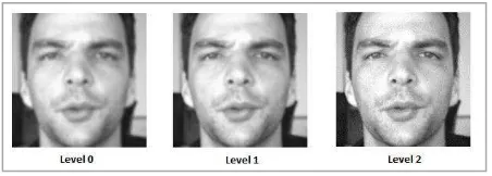
The image pyramid at the top level was the initial image. At each lower level, smoothing was applied using Gaussian Blur. It is an image convolution using Gaussian kernel. The calculation of kernel size used the equation (10) and the development of kernel Gaussian used the equation (11). Next, downsampling applied at the image resulted from smoothing was used for making the size of the image smaller. At each lower level, the size was getting diminished and the level of image clarity decreased. In Figure 1 and 2, the image at level 0 (the lowest level) was the image having the smallest size compared to its higher level. This image also had the lowest level of sharpness compared to its higher level.
Figure 1. Pyramid of Images with Actual Size in one of Images in the BioId Dataset
Figure 2. Pyramid of Images with Image Size at Each Level Equated with the Top Level of Image Size (Level 2) in one of Images in the BioId Dataset
(10)
Where
ksize is the kernel size and σ is sigma. x, Kernel index at axis x
y, kernel index at axis y in the midpoint kernel located at x = 0 andy = 0
σ, sigma value,
G(x,y), kernel value at index x and y.
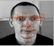
2. Patch Extraction in the Landmark area.
Figure 3. Area of Image Patch at One of Images in BioId Dataset
3. HOG feature extraction.
The extraction process of HOG features or HOG descriptors is performed on the entire patch images of the previous process. Each training data sample results in some HOG descriptors which are in accordance with the numbers of patch images and combinations of those all descriptors are used as regression training data in the next process. In short, the
formation of HOG features by extracting histogram cells’ voting values of each pixel in those
cells based on L2-norm gradient, with histogram channels, is known as orientation-based channels [9].
The extraction process of a HOG descriptor refers to [10]. This process begins with the calculation of a gradient image on axis x and y by performing convolutive operation on the image with kernel [-1,0,1] and kernel [[-1], [0], [1]]. The image in this process is a patch image resulted from the previous process. After the gradient value is resulted, calculation is performed to obtain image magnitude and gradient orientation by using equations 12 and 13.
| | √ (12)
(13)
Where,
|G| is gradient image magnitude,
Ixis gradient image resulted from convolution of axis x, Iyis gradient image resulted from convolution of axis y, θ is gradient image orientation.
The next step is developing histogram channels. Histogram channel is a histogram based on gradient image orientation angles. Each channel width or range is obtained from the division of 180 with parameter of channel numbers. Histogram channel development starts by dividing an image into some cells with the same sizes.The gradient magnitude of each cell is calculated at the channel value of that gradient orientation site. The next step is block normalization. This process starts by classifying n x ncell into the blocks. Blocks located overriding the other blocks or blocks 50% override the previous blocks that a cell may be located in two blocks or more. The results of block normalization may be obtained from equation 3:16 and all normalization results form HOG descriptors.
√‖ ‖ (14)
With, n is block normalization and v is histogram vector of all cells in the blocks. 4. Linear regression
This process aims to obtain weight of HOG features on each element of a face shape. A face shape element is one of two coordinates, that is, coordinate x or y of a landmark point. So, the number of face shape elements is twice of that of landmark points. The wieght resulted is used in fitting process.
value on each patch image around landmark point areas. While the target value or Y is the difference between GTS positions with the present face shape positions on particular face shape elements.
5. Updating the present face shape level.
This process aims to update the present face shape on a training data into face shape at SDM next level or estimation of final face shape if SDM level is the final level.This process is performed by obtaining estimation of distance changes by multiplying the weight of HOG descriptors resulted from a linear regression with the value of HOG descriptors resulted from those training data samples. Each face shape element has HOG descriptor weight and is used to obtain estimation of those shape element changes.
6. Iteration for the next SDM level
The next step is iteration of step 2 to 5. After face shape updating process, the face shape is adapted as a face shape for the next SDM level and pyramidal image is also used in the next level which is larger and clearer. Once the training phase is completed, HOG descriptor weight is resulted at each SDM level for each required face shape element for a fitting stage.
2.3. Fitting Stage
This stage aims to obtain estimation of a face shapeof an image or video. In general, fitting stage goes through several steps:
1. Detecting a face and transforming an image that the results of face detection approaching the average face detection result. The average detection result is obtained from pre-training phase. This aims to normalize the face size in the image.
2. Extracting image on face area.
3. Developing an image pyramid on face area image with a parameter of pyramid image revival based on parameter at the training stage.
4. Reviving an initial face shape as the present face shape level. The initial face shape level is obtained from the pre-training stage.
5. Extracting the entire patch image on an area around the present face shape landmark on the pyramidal image.
6. Calculating HOG descriptor value of all image patches.
7. Calculating estimation of the present distance level changes for all face shape elements. The estimation is obtained by multiplying the corresponding HOG shape element weight with the obtained HOG descriptor.
8. Updating a face shape using estimation of distance changes and adjusting the face shape as the next level face shape or the final face shape estimation result.
9. Repeating step 5 to 8 for all SDM next levels.
After completing the entire processes, filtering is performed on face shape estimation
result to obtain a stable face shape movement on video. The filtering method used is 1€ filter [11]. 1€ filter is a filter based on low-passfilter which is able to adapt the filter result based on event. Event on face alignment problems is in the form of fast and slow face movement. When
the face movements are fast, 1€ filter increases the cut off frequency value to reduce lag effects
or delayed face shape movements to follow the real face and when the face movements are
slow, 1€ filter reduces the cutoff frequency value that jitter effects or irregular movements are
reduced. Equations 15-18 are equations used in filtering process of 1€ filter.
, is sampling period,
is cut off frequency parameter , ̂, is filter result value on sample, ̂̇, is filtered derivative value,
Each sample value of coming in a time period of ,, low-pass filter is performed at a distance change difference of ̂̇which is a value difference of with ̂ and low-passfilter is performed at that distance change diference. ̂̇ Influences the formation of , the higher the value of ̂̇ the higher the value of and the lower the value of ̂̇ the lower the value of . the higher the value of the bigger the part of and the smaller the part of ̂ used for the final result of filter ̂ . on the other hand, the smaller the value of the smaller the part of and the bigger the part of ̂ influencing the filter final result. Parameter and have a clear conceptual relationship, if the problem of lag is on high speed, the value level is and if the problem of jitter is on low speed, the value of should be lowered.
3. Results and Discussion
Testing is conducted to examine the influence of some training parameters upon a face alignment accuracy level. The test is performed on BioID dataset consisting of 1521 grayscale images with the size of 384x286 pgm format obtained from a URL address: https://www.bioid.com/About/BioID-Face-Database.
A thousand images are randomly taken as training data and the rest of images are as test data. The face alignment accuracy level process is measured from the average value of RMSE (Root Mean Squared Error) between face shape estimation and on GTS dataset testing with a face size corresponding to the average detection results obtained on pre-training stage. Testing is conducted on patch-size parameter, the number of HOG channels, clusters, and downsample.The graphics in figure 4 to 8 have axis labels in the form of face shape elements and ordinate labels which are the values of RMSE resulted from harmonization of face shape on "BioID"dataset testing.
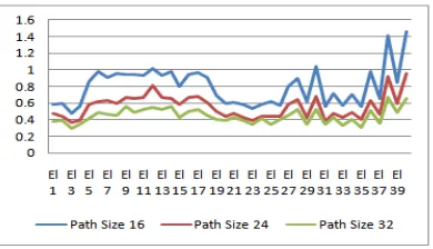
1. Patch-image size Parameters
The graphic in Figure 4 shows the influence of patch size upon SDM accuracy level. From those three value comparisons of patch size and face alignment, the 32 patch size value gives the best accuracy level. The larger the patch size the more the features are resulted from the extraction process of HOG descriptors and the more image information is obtained. The more image information tends to have better training results.
Figure 4. The Graphic of Some Patch Sizes’ Influences on SDM Accuracy
2. HOG channel number Parameters
The graphic in Figure 5 shows HOG channel numbers’ influence on SDM accuracy.
Figure 5. The Graphic of HOG Channel Number Values’ Influences on SDM Accuracy
3. Cluster number Parameters
The graphic in Figure 6 shows the influence of cluster number on SDM accuracy level. This parameter is related to sample number parameters and sample number used is 20. The highest RMSE value is obtained by cluster number which is same with sample number of 20. Cluster number of 40 and 60 give similar RMSE. This is due to the fewer spreading cluster number or cluster wide area and on the other hand, the greater the value of this parameter is centralized in the cluster area or the cluster area is not so broad that the cluster midpoint may represent better values of the cluster members. Clusters with not too spacious area tend to give revival face shape sample results approaching most GTS in dataset and the face alignment accuracy level may give better results.
Figure 6. The Graphic of Some Cluster Number Values’ Influences on SDM Accuracy
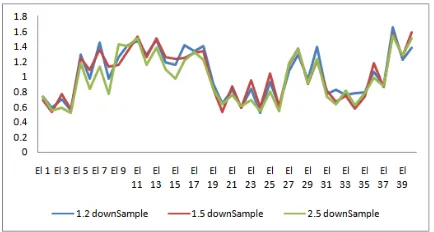
4. Downsample Parameters
The graphic in Figure 7 shows the downsample values’ influence on SDM accuracy level. Downsample influences the revival of pyramidal images at each SDM.Thesmaller the value of downsample, the larger, clearer, more detail the piramidal image on each SDM level.
Those three graphics in Figure 7 represent similar values. The greater or the smaller the value of downsample does not ensure the increase of the alignment face accuracy. The best Value of downsample may be obtained through testing.
4. Conclusion
The ability of this modified SDM method gives quite good results in solving face alignment on BioID dataset. The use of this method with cluster number parameter values which are twice or three times of the sample number parameter values gives more accurate face alignment results than with cluster number which is only once of the sample value. The size of image patch with a value of 32 results in more accurate estimation of face landmark than with the patch size of 16 and 24.HOG channel number of 9, 13, 17 and 21 do not significantly give different face alignment accuracy. The downsample value of 1.5 gives more accurate face alignment than downsample of 1.2 and 2.5 however, the difference is not too significant. The recorded best accuracy level in testing process of BioID dataset, RMSE mean is measured with the value of 0.881693525. A suggestion for further development is that in further testing of feature extraction process, other methods, such as SURF, FAST, and ORB may be used.
References
[1] Wu H, Liu X, Doretto G. Face Alignment via Boosted Ranking Models. IEEE Conference on Computer Vision and Pattern Recognition. Anchorage, Alaska. 2008: 1-8.
[2] Su Y, Ai H, Lao S. Real-Time Face Alignment with Tracking in Video. 15th IEEE International Conference on Image Processing. California. 2008: 1632-1635.
[3] Jiao F, Li S, Shum HY, Schuurmans D. Face Alignment using Statistical Models and Wavelet Features. IEEE Computer Society Conference on Computer Vision and Pattern Recognition. Wisconsin. 2003: 321-327.
[4] Wang W, et al. An Improved Active Shape Model for Face Alignment. 4th IEEE International Conference on Multimodal Interfaces. Pennsylvania. 2002: 523-528.
[5] Budiharto W, Santoso A, Purwanto D, Jazidie A. Multiple Moving Obstacles Avoidance of Service Robot using Stereo Vision. TELKOMNIKA. 2011; 9(3): 433-444.
[6] Xiong X, De la Torre F. Supervised Descent Method and Its Applications to Face Alignment. IEEE Conference on Computer Vision and Pattern Recognition. Oregon. 2013: 532-539.
[7] Chuan L, et al. Face Detection Algorithm Based on Multi-orientation Gabor Filters and Feature Fusion.
TELKOMNIKA. 2013;11(10): 5986-5994.
[8] Shamsudin SA. A Closed-Form Solution For The Similarity Tranformation Parameters Of Two Planar Point Sets. Journal of Mechanical Engineering and Technology (JMET). 2013; 5(1): 59-68.
[9] Hamid O, Mohammed O. Aksasse B. Gabor-HOG Features based Face Recognition Scheme.
TELKOMNIKA. 2015;15(2): 331-335.
[10] Dalal N, Triggs B. Histograms of Oriented Gradients for Human Detection. IEEE Computer Society Conference on Computer Vision and Pattern Recognition. Caifornia. 2005: 886-893.