CHAPTER 2 LITERATURE REVIEW
2.1 Artificial Neural Network
Artificial neural network (ANN), usually called Neural Network (NN), is an
algorithm that was originally motivated by the goal of having machines that
can mimic the brain. A neural network consists of an interconnected group of
artificial neurons. They are physical cellular systems capable of obtaining,
storing information, and using experiential knowledge. Like human brain, the
ANN’s knowledge comes from examples that they encounter. In human
neural system, learning process includes the modifications to the synaptic
connections between the neurons. In a similar way, ANNs adjust their
structure based on output and input information that flows through the
network during the learning phase.
Data processing procedure in any typical neural network has two major steps:
the learning and application step. At the first step, a training database or
historical price data is needed to train the networks. This dataset includes an
input vector and a known output vector. Each one of the inputs and outputs
are representing a node or neuron. In addition, there are one or more hidden
layers. The objective of the learning phase is to adjust the weights of the
connections between different layers or nodes. After setting up the learning
samples, in an iterative approach a sample will be fed into the network and 2.1 Artificial Neurarall Network
Artifificicial neural l neetwtwork (AANNNN),) usuu ualllyly ccalalleledd Neural Netwowork (NN), is an a
algorithm m ththat wasa originaallllyy momotitivavatetedd byby the goao l off hhavaving machc ines that can n mimimmiccthe brbrain. A neural network consists of anan interrcoconnnneected grouo p of ar
artiifificial nneurons. They are physical cellular systems capapablel oof f obtainining, st
sorinng information, and using experiential knowledge. Like huhumaan brbraiainn, thee ANNN’s knowledge comes from examples that they encounteer. In n huhuman n
neeural system, learning process includes the modifications to tthe synappticc coonnections between the neurons. In a similar way, ANNs aadjuustst theirir structure babasesedd onon ooututpuput t anand inpuputt ininfoformrmatatioionn ththatat flows through thehe network during the learning phase.e
Da
Datatapprorocecessssiningg prprococededururee ininaanyny typypicicalal nneueurarallnenetwtworork khahass twtwoomamajojorr ststeps: th
the resulting outputs will be compared with the known outputs. If the result
and the unknown output are not equal, changing the weights of the
connections will be continued until the difference is minimized. After
acquiring the desired convergence for the networks in the learning process,
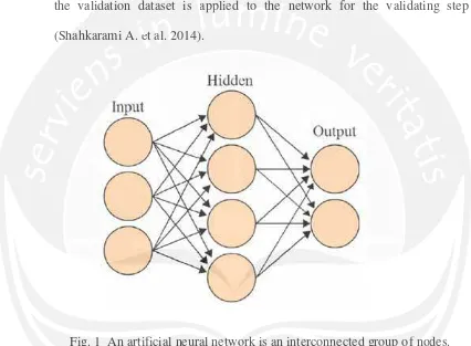
the validation dataset is applied to the network for the validating step
(Shahkarami A. et al. 2014).
Fig. 1 An artificial neural network is an interconnected group of nodes.
Source : SPE International, Colorado, USA, 16–18April 2014.
2.2 Review of previous researches
Several economists advocate the application of neural networks to different
fields in financial markets and economic growth methods of analysis (Kuan,
C.M. and White, H. 1994). We focus the review of prior studies on prediction
of financial market. Chen et al (2003) attempted to predict the trend of return connections will be coontntininued until l ththe e difference is minimized. After acquiring the dedesired convergence for the networksks in the learning process, the valiidadation dataset is aapplpieied d toto tthee network for tthehe validating step (SShahahkarami A.eet alal. 22014).
Fig.11 AAn arartitifificicial neurall l nenetwtworork k isis an intercrcononnenected group of d fnonodedes. S
Sourcee:: SPSPE Internatioonan l, Colorraado, USA, 166––1818ApAp irill 20201414.
2.2 Review of previous researchhese
on the Taiwan Stock Exchange index. The probabilistic neural network
(PNN) is used to forecast the trend of index return. Statistical performance of
the PNN forecasts is compared with that of the generalized methods of
moments (GMM) with Kalman filter and random walk. Empirical results
showed that PNN demonstrate a stronger predictive power than the GMM–
Kalman filter and the random walk prediction models. Kim (2003) used SVM
to predict the direction of daily stock price change in the Korea composite
stock price index (KOSPI). This study selected 12 technical indicators to
create the initial attributes. The indicators are stochastic K%, stochastic D%,
Slow %D, momentum, ROC, Williams’ %R, A/D oscillator, disparity 5,
disparity 10, OSCP, CCI and RSI. In addition, this study examined the
feasibility of applying SVM in financial prediction by comparing it with
back-propagation neural network (BPN) and case-based reasoning (CBR).
Experimental results proved that SVM outperform BPN and CBR and
provide a promising alternative for stock market prediction. Altay & Satman
(2005) compared the forecasting performance artificial neural network and
linear regression strategies in Istanbul Stock Exchange and got some evidence
of statistical and financial outperform of ANN models. Kumar & Thenmozhi
(2006) investigated the usefulness of ARIMA, ANN, SVM, and random
forest regression models in predicting and trading the S&P CNX NIFTY
Index return. The performance of the three nonlinear models and the linear
model are measured statistically and financially via a trading experiment. The the PNN forecasts is comompared withh tthahat of the generalized methods of moments (GMMMM)) with Kalman filter and random m walk. Empirical results showedd tthhat PNN demonstrtrattee a a ststrorongngerr ppredictive poweer r than the GMM– Kaalmlman filter anndd ththe rrandom walk predictionon mmododeels. Kim (200303))used SVM to preedidictct ttheh direcectition of daily stock price chchanange in n ththee KoK rea coompm osite st
stocockk pprice e iindex (KOSPI). This study selected 12 tetechniicaal l inindidicatorsrs to create tthhe initial attributes. The indicators are stochastic K%%, stoochchasastic D%%, Sloww %D, momentum, ROC, Williams’ %R, A/D oscillatorr, disispaparirityt 5, dissparity 10, OSCP, CCI and RSI. In addition, this study exxamined ththee feeasibility of applying SVM in financial prediction by comparring it withh ba
backc -propagationn nneueurarall nen twork (BPNN)) anandd cacasese-based reasonininng (CBBRR). Experimental results proved ththatt SSVM outperform BPN and CBR R anandd pr
provo ide a promising alternative for stock market prediction. Altayay && SSatatmam n (2
( 0005)5) comparered d ththee forecaaststiningg peperfrfoormance e arartitifificiial neural ll netwtwororkk and li
linenear reggreressssioion strategies innIIstanbul SStock Exchangeeaandndggotsomome evidence of statistical and financial ouutperform oof ANN models. Kumar & Thenmozhi (2006) investigated the usefefulness off ARIMA, ANN, SVM, and random forest regression models in prredicctiting and trading the S&P CNX NIFTY
empirical result suggested that the SVM model is able to outperform other
models used in their study.
Hyup Roh (2007) introduces hybrid models with neural networks and time
series model for forecasting the volatility of stock price index in two vision
points: deviation and direction and the results showed that ANN-time series
models can increase the predictive power for the perspective of deviation and
direction accuracy. His research experimental results showed that the
proposed hybrid NN-EGARCH model could be improved in forecasting
volatilities of stock price index time series.
Adebiyi Ayodele A. et al. (2009) presented a hybridized approach which
combines the use of the variables of technical and fundamental analysis of
stock market indicators for daily stock price prediction. The study used
three-layer (one hidden three-layer) multithree-layer perceptron models (a feedforward neural
network model) trained with backpropagation algorithm. The best outputs of
the two approaches (hybridized and technical analysis) are compared.
Empirical results showed that the accuracy level of the hybridized approach is
better than the technical analysis approach. Liao & Wang (2010) applied a
Stochastic Time Effective Neural Networks in predicting China global index
and their study results showed that the mentioned model outperform the
regression model. Kara et al (2011) compared neural networks performance
and SVM in predicting the movement of stock price index in Istanbul Stock
Exchange. The input variables in suggested models include technical
indicators such as CCI, MACD, LW R%, etc. The results revealed that neural Hyup Roh (2007) inntrtroduces hybrid modelsls wwith neural networks and time series modell ffor forecastingg the volatility of stock priricec index in two vision pointss:: deviation n annd d directtioion ann a d d ththe reresusultltss showed that ANA N-time series m
models canan increasase the predicictitiveveppowower for thepperspecective of devivation and direectctioion n accuraracy. His research experimental l reresults s shshowowed thahat the pr
propoposed hhybrid NN-EGARCH model could be improovev d inin fforecastiting vo
v latiillities of stock price index time series.
Addebiyi Ayodele A. et al. (2009) presented a hybridized apprproachch wwhichch coombines the use of the variables of technical and fundamental analysiiss oof stoock market indicators for daily stock price prediction. The studyy ususeed threeee- -layer (one hidden -layer) mulultitilalayer pepercrceptron models (a feedforward neueuraral
network model) trained with backpropagation algorithm. The best oouutpuputsts of th
thee twtwoo apapprproaoachches ((hyhybrbrididizized andand ttecechnhniicalal aananalylysisis)s) aarere comompapared. Em
networks work better in prediction than SVM technique. Zhou Wang et al
(2011), propose a new model to predict the Shanghai stock price. They used
Wavelet De- noising- based Back propagation (WDBP) neural network. For
demonstrating superiority new model in predicting, the results of it is
compared with Back Propagation neural network and the total results showed
that the WDBP model for forecasting index is better than BP model.
Putra and Kosala (2011) try to predict intraday trading Signals at IDX they
used technical indicators - the Price Channel Indicator, the Adaptive Moving
Averages, the Relative Strength Index, the Stochastic Oscillator, the Moving
Average Convergence-Divergence, the Moving Averages Crossovers and the
Commodity Channel Index. The result of their experiments showed that the
model performs better than the naïve strategy. Also Veri and Baba (2013)
forecasting the next closing price at IDX, they used opening price, highest
price, lowest price, closing price and volume of shares sold as experimental
variables. The result showed that the most appropriate network architecture
is 5-2-1 with dividing the data into two parts, with 40 training data with 95%
accuracy of data and 20 test data with 85% accuracy of data.
2.3 Learning Paradigms in ANNs
The ability to learn is a peculiar feature pertaining to intelligent systems,
biological or otherwise. In artificial systems, learning (or training) is viewed
as the process of updating the internal representation of the system in
response to external stimuli so that it can perform a specific task. This Wavelet De- noising- basaseded BBack propagagataion (WDBP) neural network. For demonstrating g susuperiority new model in predictctining, the results of it is compareded with Back Propaaggatitiononnneueuraral lnenetwork and the tototat l results showed thatat the WDBP mom ddel l for forecasting index isis bbetetteterr than BP modedel.
Putrra a anandddd Kosalalaa (2011) try to predict intraday ttradiradng SSigignanalsl at IDDX X they us
useded technhnical indicators - the Price Channel Indicator, thehe Adadaptptivive Moviving Av
A eraages, the Relative Strength Index, the Stochastic Oscillatator, ththe MoMovingg Aveerage Convergence-Divergence, the Moving Averages Crossooversrs aandnd the Coommodity Channel Index. The result of their experiments showwed that tthee m
model performs better than the naïve strategy. Also Veri and BBaba ((2013)3) forecastinng g ththee nenextxt cclolosisng price at IDp IDX,X, ttheheyy ususeded oopepening price, highghesestt price, lowest price, closing pricee aand volume of shares sold as experirimementntaal va
v riiabableless. ThThee reresusultlt sshohowewed that the mmosostt apapprpropopririatatee netwnetworkk ararchchititecectture is
is55-2-1 wwitithh didivividiingngttheheddata inintoto ttwo pparartsts, wiwithh440 0 trtraiaining ddatata a wiwithth 95% accuracy of data and 20 test ddaata withh885% accuracy of data.
2.3 Learning Paradigms in ANNNs
The ability to learn is a peculiliar ffeature pertaining to intelligent systems,
includes modifying the network architecture, which involves adjusting the
weights of the links, pruning or creating some connection links, and/ or
changing the firing rules of the individual neurons.
ANN approach learning has demonstrated their capability in financial
modelling and prediction as the network is presented with training
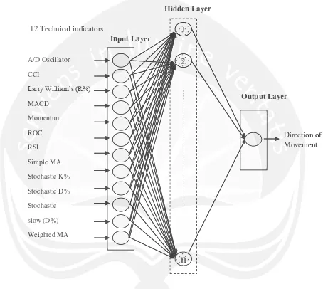
examples, similar to the way we learn from experience. In this paper, a
three-layered feed-forward ANN model was structured to predict stock price
index movement is given in Fig. 2. This ANN model consists of an input
layer, a hidden layer and an output layer, each of which is connected to the
other. At least one neuron would be employed in each layer of the ANN
model. Inputs for the network were twelve technical indicators which were
represented by twelve neurons in the input layer. Each neuron (unit) in the
network is able to receive input signals, to process them and to send an
output signal. Each neuron is connected at least with one neuron, and each
connection is evaluated by a real number, called the weight coefficient, that
reflects the degree of importance of the given connection in the neural
network (Daniel et al. 1997).
The error between the predicted output value and the actual value is
back-propagated through the network for the updating of the weights. This
method is proven highly successful in training of multi-layered neural
networks. The network is not just given reinforcement for how it is doing on
a task. Information about errors is also filtered back through the system and changing the firing rules ofoftthhe individuaall nen urons.
ANN apprprooach learning g has demonstrated their ccapa ability in financial modedellling and d prprede ictionon ass ththee nen twtworork k is presenteded with training exampleses, similalar to the wayay wwee lelearn from eexpx erieencn e. In thhisis paper, a threree-e-lalayey red fefeed-forward ANN model was strucctutured tooppreredidct stockck price innded x momovement is given in Fig. 2. This ANN model coc nsisiststs oof an inpnput layeerr, a hidden layer and an output layer, each of which is coconnneecteed d tot thee otthher. At least one neuron would be employed in each layerr of ththee ANA N m
model. Inputs for the network were twelve technical indicators which wweeree r
represented by twelve neurons in the input layer. Each neuron ((unit)t) in thhe network isis aablblee toto rrececeieve iinput sigignalss,, toto pprorocecessss ttheh m and to sendd anan output signal. Each neuron is coonnn ected at least with one neuron, anndd eaeacch connnecectitionon iiss evevalaluauatetedd byby a real numbberer,, callcallededtthehewweieighghtt coefffificicienent,t,tthat re
reflects tthehe ddegegreeee ofof iimpm ortatancncee of tthehe ggivivene ccononnenection inin tthehe neural networkk (Daniel et al. 1997).).
is used to adjust the connections between the layers, thus improving
performance.
Fig. 2. A Neural network with three-layer feed forward
Source: Y. Kara et al. / Expert Systems with Applications 38 (2011)
5311–5319
This a supervised learning procedure that attempts to minimise the error
between the desired and the predicted outputs. If the error of the validation
A/D Oscillator
Fig. 2. A Neural network with three-layer feed forward
Source: Y. Kara et al. / Exppert Systemms with Applications 38 (2011) 5311–5319
This a supervised learning procedure that attempts to minimise the error A/D OOscillator
12 Technical indndicators 1
patterns increases, the network tends to be over adapted and the training
should be stopped.
The most typical activation function used in neural networks is the logistic
sigmoid transfer function. This function converts an input value to an output
ranging from 0 to 1. The effect of the threshold weights is to shift the curve
right or left, thereby making the output value higher or lower, depending on
the sign of the threshold weight. The output values of the units are
modulated by the connection weights, either magnified if the connection
weight is positive and greater than 1.0, or being diminished if the connection
weight is between 0.0 and 1.0. If the connection weight is negative or (value
< 0) then tomorrow close price value < than today’s price (loss). If (value >
0.5) then then tomorrow close price value > than today’s price (profit). As
shown in Fig. 2, the data flows from the input layer through zero, one, or
more succeeding hidden layers and then to the output layer. The
back-propagation (BP) algorithm is a generalisation of the delta rule that works
for networks with hidden layers. It is by far the most popular and most
widely used learning algorithm by ANN researchers. Its popularity is due to
its simplicity in design and implementation. The idea is to train a network
by propagating the output errors backward through the layers. The errors
serve to evaluate the derivatives of the error function with respect to the
weights, which can then be adjusted. It involves a two stage learning process
using two passes: a forward pass and a backward pass. The basic back
propagation algorithm consists of three steps (Fig. 2). Although, the most The most typical actctivivation function used inin nneural networks is the logistic sigmoid tranansfer function.. This function converts aniinpnput value to an output ranggining from 00 to 1.1 Theeefffecectt ofofttheh tthrhresshohold weights is toto shift the curve right or llefe t, theererebyb making g ththee ououtptput value hhigigher orr lower, depepending on thee sisigngn of ththe threshold weight. The outputut values s ofof the uninitst are mo
modulateted by the connection weights, either magnifieed d if tthehe cconnecttioi n weigghht is positive and greater than 1.0, or being diminishedif ifthe ecoconnnnece tionn we
weight is between 0.0 and 1.0. If the connection weight is negatative oor ((vav lue <
<0) then tomorrow close price value < than today’s price (loss)). If (valuuee>> 0
0.5) then then tomorrow close price value > than today’s price (profofiit). AAs
shown inn FFigig.. 2,2, thethe ddataa flflowo s fromom thee iinpnputut llayerayer tthrh ough zero, onee,, oror more succeeding hidden layerss and then to the output layer. The e baback ck-pr
poppagagatatioionn (B(BP)P) aalglgororitithmhm is a generaralilisasatitionon ooff ththee dedeltltaa rule tthahat t woworks fo
(i = 1,2,…n) (1)
(2)
(3) commercial back propagation tools provide the most impact on the neural
network training time and performance. The output value for a unit is given
by the following Equation:
Where y the output value is computed from set of input patterns, Xi of ith
unit in a previous layer, Wij is the weight on the connection from the
neuron ith to j,ࣂ j is the threshold value of the threshold function f, and n is
the number of units in the previous layer. The function ƒ(x) is a sigmoid
hyperbolic tangent function (Barndorff-Nielsen et al. 1993)
ࢌሺ࢞ሻ ൌ ሺݔሻ ൌ ଵିଵାషష Threshold: ݂ሺݔሻ ൌ ቄͲͳ௧௪௦௫ழǡଵ
where ƒ(x) is the threshold function remains the most commonly applied in
ANN models due to the activation function for time series prediction in
back-propagation (Najeb Masoud, 2014): by the following Equatioionn:
(4)
(5) Once the output has been calculated, it can be passed to another neuron (or
group of neurons) or sampled by the external environment. In terms of the
weight change, Δwij, the formula equation is given as:
ο࢝ ൌ ࣁࢾ࢞
where ηis the learning rate (0<η<1), δjis the error at neuron j,xi is an input vector and withe weights vector. This rule of IDX can also be rewritten as:
ο࢝ ൌ െࣁሺ࢚െ ࢞࢝ሻ࢞
Although a high learning rate, η, will speed up training (because of the large
step) by changing the weight vector, w, significantly from one phase to
another. According to Wythoff BJ. (1993) suggests that η[0.1,1.0]. (4)
(55)) weight change, Δwij, the e foformula equatitionon is given as:
ο࢝ ൌ ࣁࢾࢾ ࢞
wh
whereηis thelleaearrnining ratee((0<0<η<<1)), δδjδ isistthehe eerrrroror at neuron jj,xxi is an input vectorraandnd withe weweigighhts vector. This rulle eofof IDX cannaalslsoo be rewriritten as:
ο
ο࢝࢝ ൌ െࣁሺ࢚െ ࢞࢝ሻ࢞
Althhough a high learning rate, η, will speed up training (becauause of f ththee largee sttep) by changing the weight vector, w, significantly from oone pphahasse ttoo a