DOI: 10.12928/TELKOMNIKA.v13i2.1437 632
An Ant Colony-Based Heuristic Algorithm for Joint
Scheduling of Post-Earthquake Road Repair
and Relief Distribution
Bei Xu, Yuanbin Song*
Department of Transport, Shipping and Logistics, Shanghai Jiao Tong University, Shanghai 200240, China
*Corresponding author, e-mail: [email protected]
Abstrak
Emergency road repair and distribution of relief goods are crucial for post-earthquake response. However, interrelationships between those two tasks are not adequately considered in their work schedules, especially in cases with very limited repair resources, leading to unnecessary delay and expenditure. A time-space network model is constructed to better describe the constraints arising from the interrelationships in joint scheduling of road repair and relief distribution works. An ant colony-based Heuristic algorithm is developed to solve the NP-hard model efficiently for practical use, followed by a case study of Wenchuan Earthquake to validate the planning tool and to demonstrate its feasibility for resolving real world problem.
Keyword: Ant Colony Algorithm, Scheduling, Post-earthquake Response, Time-Space Network
1. Introduction
Earthquake is considered as a serious threat to life safety. To reduce life loss and injuries, the delivery of living and medical commodities to beneficiaries is the most urgent and important work in the short-term post-earthquake response. The distribution efficiency is greatly dependent on the recovery of road network. Unfortunately, cases often occur that repair resources are too limited to repair all the damaged roads in a short time. Thus a short-team repair plan for part of the damaged road segments, as well as a corresponding delivery plan, has to be made on purpose of improving the relief distribution efficiency.
However, great challenges still exist to optimize the efficiency. On the term of practice, road repair and relief distribution work are now scheduled manually and separately by different departments according to decision-makers’ experience in China. As for researches related, up to now, while post-earthquake road repair and relief distribution are extensively researched respectively, the study of joint scheduling of post-earthquake road repair and relief distribution remains at a low level. It is also recognized by Altay and Green [1] that the lack of research on incorporate operations would be the bottleneck in the field of disaster response. To the best of our knowledge, there are few researches on joint scheduling of post-earthquake road repair and relief distribution. Yan and Shih present the first significant research that directly targets this issue [2]. They establish a multi-objective mixed-integer model of time-space network to minimize the time necessary for both road repair and relief distribution in 2009. A heuristic algorithm with Cplex is developed for solving such models to limit the solution time in a reasonable and practical range. Later in 2012 and 2014, the optimal scheduling of logistical support for emergency roadway repair work is further studied as a supplement for the previous research [3],[4]. However, serious limitations still exist in these models due to some over idealistic assumptions. The number of damaged points on the same road segment is limited to no more than two while three or more may occur in real cases, especially on a twist long mountain road. The impact of post-earthquake bad weather on repair efficiency is not considered, which may greatly influence road repair and relief distribution schedules.
2. Model and Method
2.1. Time-space Network Model
To model the realistic problem, some assumptions are made as below.
a) A short-term repair and relief distribution plan is considered, which requires for a quick and reliable plan on the main purpose of distributing relief materials to all beneficiaries.
b) Bad weather reduces the repair work efficiency of damaged points by different degrees. Two types of damaged points are considered: weather sensitive (flooded by quake lake, buried by landslides) and insensitive (blocked by rocks, destroyed by crustal deformation). The efficiency decay rate of either type is given according to historical experience.
c) All the geographic and operation information is known.
d) Work teams do not need to return to their work stations. The rescue machinery, fuel and other resources will be supplied to the work teams by support units.
e) Only commodity flows are considered in the relief distribution network.
f) Every damaged point can be repaired by no more than one work team. All work teams are assumed to be equivalent in terms of repair efficiency.
g) Multiple damaged points (>2) are allowed on the same segment. Damages at intersections are also considered.
h) To simplify the distribution model, relief materials like clothes, water, food, medicine and tents are all packed and calculated as equivalent relief units.
i) A minimum percentage of each demand point’s overall demand is considered when allocating commodities in the case of supply shortage.
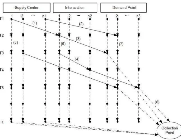
Firstly, two similar networks are established for road repair and relief distribution respectively in Figure 1 and Figure 2. Every node in the time-space networks has dual attributes. The horizontal axis represents its space attribute as a location like work station, intersection, damaged point, supply center or demand point. The vertical axis represents its time attribute of the location’s state at a specific moment. Every arc represents a work team flow or a commodity flow. Collection points are virtual points used to ensure the flow conservation.
Figure 2. Relief distribution time-space network (RDTN)
In this model, max out-flow of each work station equals to its origin number of available work teams. Max out-flow of each supply center equals to its origin amount of available supply. Max out-flow and max in-flow of each damaged point are both set to be 1. Max in-flow of each demand point equals to its total amount of demand. Infinit out-flow and in-flow are allowed for each intersection and the passable work teams and commodity are also infinite on each road segment. Different arc types and their flow range in both networks are displayed in Table1.
Table 1. Arc type and flow range in time-space networks.
Arc Type Flow Range Arc Type Flow Range
In RRTN In RDTN
(1) work station-intersection [0,wti] (1) supply center-intersection [0,i]
(2) work station-damaged point [0, 1] (2) supply center-demand point [0, min( i, j)]
(3) intersection-damaged point [0, 1] (3) intersection-demand point [0,j]
(4) intersection-intersection [0,] (4) intersection-intersection [0, ]
(5) damaged point- damaged point [0, 1] (5) holding arc: supply center [0,i]
(6) holding arc: work station [0,wti] (6) holding arc: intersection [0,]
(7) holding arc: intersection [0,] (7) holding arc: demand point [0,j]
(8) holding arc: damaged point [0, 1] (8) collection arc [0,]
(9) collection arc [0,]
* wti is the origin number of available work teams at the ith work station; i is the total supply of theith supply center;jis the total demand of thejth demand point.
In post-earthquake short-term emergency logistics, life injury and property damage are much more important than the repair and distribution cost of money. Considering different urgent levels of demand points, a weighted sum of the arrival time associated with every demand point in relief distribution is set as the model objective to minimize.
In modeling, i t( )represents a node in time-space network while i denotes its space attribute and t denotes its time attribute. Arc i t j t( ) ( ') then describes a work team/commodity movement from the ith location at the tth time to the j th location at the 't th time. For simplicity, a single i represents a location node at any time in time-space networks.
We can then fomulate the objective function as equation (1).
1 1
min : a i(T it ), D
i t
where eit is a binary variable; ui is the urgent level of the ith demand point; D
M is the set of all demand points; a is the number of demand point; T is the total time length of time-space network.
There are five types of constraints need to be considered in modeling. a) Flow Conservation
The time-space network model shares the similar flow conservation constraints with other network flow models as equation (2) and equation (3).
(units: commodity equivalents);NDis the set of all locations in RDTN; WS is the set of all work stations; DPis the set of all damaged points; SCis the set of all supply centers; INis the set of all intersections; INVis the set of all virtual intersections.
b) Flow Restriction
Work team arc and commodity arc are also restricted by the road network accessablity and flow upper bounds assumed in Table 1, in addition to their own properties as nonnegative integer, as formula Equation (4)-(6). variable which denotes the accessibility of arc ij in RDTN; gij is the flow upper bound of arc ij
in RRTN; sij is the flow upper bound of arc ij in RDTN; AR is the set of all arcs in RRTN; AD is the set of all arcs in RDTN.
To model the problem of multi damaged points on one segment, a damaged point at a
-way intersection is extended to virtual damaged points with the same workload and damage type on the adjacent segments and a virtual intersection is inserted between two adjacent damaged points to cut the original segment into several sub-segments with only one damaged point.
D is the set of all damaged points at intersection; PV q
D is the set of virtual damaged points extended from the th damaged point; q is the number of road segments linked to the intersection with the th damaged point.
c) Repair Work Constraints
Equation (12) ensures repair work starts once a work team arrives at a damaged point and equation (13) requires the work team to leave the damaged point once repair work finishes.
Repair work efficiency is assumed to change with different weather conditions over time, which makes it a time-dependent factor. It is linearly formulated as equation (14) for simplicity. And the repair time is determined by the time associated with the start node as equation (15).
E is the repair efficiency of the th damaged point in good weather condition; t q E is the repair efficiency of the qth damaged point at the tth time after earthquake; DPW is the set of all weather sensitive damaged points; bwt is the predicted bad weather index at the tth time after earthquake; bws is the safe threshold of bad weather index; q is the repair efficiency decay parameter of the qth damaged point, q [0,1]; WLq is the total workload of the qth damaged point.
Equation (16) ensures that a damaged point could be repaired by no more than one work team and allows repairing only some of the damaged points.
( ) 1,
To avoid serious insufficiency, the sum of all commodity arc flows to each demand point should not be less than the minimum percentage of its demand, as formulated in equation (17).
Equation (18) ensures that positive collection arcs are allowed only if the minimum required demand of a demand point is met and equation (19) records the demand met time.
( ') ( ') ( ')
where M is a very large positive number; DCP
N is the set of collection point in RDTN.
Equation (20) ensures that no more commodity is delivered to a demand point after its minimum demand is met.
Equation (21) clears all the arc flows in RRTN and RDTN after the minimum demand of all demand points are met, which means the repair and the distribution work are all finished.
1
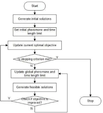
The time-space network model is formulated as a mixed-integer multi-commodity network flow problem, which is characterized as NP-hard. It is difficult to optimally solve in a limited time for large problems. Therefore, we develop a hybrid global search Heuristic algorithm to efficiently solve the problem by applying the pheromone idea of ant colony system algorithm.The algorithm framework is shown in Figure 3.
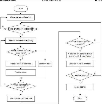
Initial and feasible solution method
The process to generate a feasible solution is framed in Figure 4. Firstly, a work team is randomly chosen to make an action decision at the beginning of a time unit that whether it would stay still, travel to an adjacent intersection or start to repair a damaged point. The decision making process follows a pseudo-random proportional rule determined by pheromone [5-7], which is formulated in equation (22).To reduce the computing scale, state check is conducted in advance that only work teams who finish their previous traveling or repairing work have to do the decision making process.
where P i j( , ) is the probability with which a work team chooses to move from node i to node
j ; p i j( , ) is the pheromone value from node i to node j ; J i( ) is the set of nodes that can be visited from node i.
Figure 3. Framework of the hybrid global search Heuristic algorithm
Figure 4. Framework of the feasible solution method
1
min : a i i
i
Z u T
(23)
Subject to
1 a b
a a k a
k
s
(24)
1 0 a bk b
k
s
(25)
1 2
max , ,...,
a a a ba
T t t t (26)
[ ba 0.5]
ba ba
ba
s
t et
s h
0sba (28)
where Ta is the time when the minimum demand percentage of ath demand point is met;tba is the arrival time of commodities from bth supply center to ath demand point;etba is the earliest arrival time from bth supply center to ath demand point calculated with Dijkstra Algorithm; sba
is the total amount of commodity allocated to ath demand point from bth supply center;ua is the urgent level of ath demand point;ais the minimum percentage of demand required for the
ath demand point; ais the total demand of ath demand point;b is the total supply of bth supply center;bis the total number of supply center.
Considering the case that a later repaired damaged point near to a demand point may improve the earliest arrival time from a supply center, a local search method is applied to find possible better solutions based on the obtained feasible solution. The decide-check process and earliest arrival time calculation are repeated for another l time units. In this period, once an earliest arrival time is shortened, the allocation model updates its solution. The optimal solution is replaced by the new one when model objective gets improved. The range of local search method is determined by the value of l.
Combining the work team paths, commodity paths and commodity allocation, we finally obtain a feasible solution for the original scheduling problem. Specifically, to improve the global search efficiency, initial pheromones and solution upper bound are set by generating a good initial solution. The initial solution method follows the feasible solution method except that work teams are always assigned to their nearest damaged point when making action decisions. Its result provides a time length limit for the repair work beyond which the solution can not be improved and a new iteration should be started to fastern the searching speed. And of course, the time length limit is updated with the improvement of optimal solutions.
Pheromone update rules
A local pheromone update rule is applied in the work team decision making process as equation (29). It cuts down the probability of pacing up and down between two points by punitively reducing the pheromone of the turn back way of a work team temporarily.
,
, , [0,1]p j i p j i (29)
where p j i( , ) is the pheromone value from node j to node i at the decision moment when a work team from node i arrives at node j ; is the pheromone decay parameter.
On the other hand, pheromones are updated globally everytime when a feasible solution is found. Equation (30) is to give higher amounts of pheromone to arcs belonging to the best solution in every iteration. Equation (31) is to decrease the pheromone level for the arcs in inferior solutions. Equation (32) is used to set the initial pheromone values.
where and are the pheromone decay parameters; Zbest and Z0 is the objective value of the current best solution and the initial solution, respectively;n is the total number of nodes in the RRTN;p0 is the initial pheromone level.
Stopping criterion
There are two stopping criteria to reduce computation time. TT is total computation time, which reflects the speed requirement in emergency condition;TI is the number of iterations since the last objective value is updated without improvement, which reflects the quality requirement of solution.
Since solutions must be found in a limited time in emergent situations, TT is set as the final stopping criterion. Sometimes when the solution quality is satisfying enough, the computation time may be far less than TT and the algorithm should stop to give early solution and save more time. Therefore, TI is set as an early stopping criterion after which the algorithm stops before meeting the final stopping criterion.
3. Numberical Test
Due to some confidential issues, the tested cases are reconstructed based on the facts of Anxian County in Sichuan Province during the 2008 Wenchuan Earthquake. Three cases of defferent scales are considered to test the algorithm performance against a direct solution with Cplex 12.5. Case A consists of 14 intersections, 16 damaged points, 1 work station, 2 supply centers and 2 demand points. Case B consists of 20 intersections, 26 damaged points, 2 work station, 2 supply centers and 4 demand points. Case C consists of 30 intersections, 36 damaged points, 3 work station, 2 supply centers and 6 demand points.These tests are performed on an Intel Pentium 4 CPU 3.2GHz with 2GB RAM under Microsoft Windows 7.
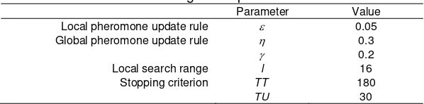
As shown in Table 2, it takes 53703.44s (about 14.9 hours), 81997.03s (about 22.8 hours) and 129663.58s (about 36.0 hours), respectively, to find the optimal solutions for tested cases directly with Cplex due to their large problem size displayed in Table 3. The Heuristic algorithm only took 93.68s and 132.70s to reach or get close enough (gap within 5%) to the optimal solution in Case A and Case B. This validates the effectiveness and efficiency of the Heuristic algorithm in solving models of middle/large scale. The relatively larger gap in Case C resulted from the stopping criterion settings in Table 4. The Heuristic algorithm stopped when the final stopping criterion was met at 180s in Case C with an objective that still could be improved. Therefore, if allowed, a bigger l can be used to improve the solution quality when the algorithm is applied in very large-scale cases.
Table 2. Test result
Cplex 12.5 Heuristic Algorithm
Case A
Number of Repaired Damaged Points 8 8
Objective 138 138
Gap (%) 0.00 0.00
Computation Time (s) 53703.44 93.68
Number of iterations - 81
Case B
Number of Repaired Damaged Points 17 17
Objective 318 330
Gap (%) 0.00 3.77
Computation Time (s) 81997.03 132.70
Number of iterations - 96
Case C
Number of Repaired Damaged Points 23 25
Objective 732 797
Gap (%) 0.00 8.88
Computation Time (s) 129663.58 180.00
Table 3. Problem size.
Local pheromone update rule 0.05
Global pheromone update rule 0.3
0.2
Local search range l 16
Stopping criterion TT 180
TU 30
4. Conclusion
To solve the joint scheduling problem of post-earthquake short-term road repair and relief distribution in repair resource shortage condition, a time-space network model is established in this paper, considering the weather factors’ and demand urgent level’s influence on damaged point selection. It could be used to find optimal routes and schedules for both road repair work teams and relief commodity flows in the same framework. This model differs from the previous ones mainly in three aspects. (1) It could be succinctly and effectively employed in complex situations with more than two damaged points on the same segment as well as damaged points at intersections. (2) Weather related factors like road damage type, repair efficiency and bad weather condition are for the first time taken into consideration to generate a more appropriate to-repair damaged point selection when the available repair resources are too limit to waste in repairing unnessary segments. (3) Urgent levels of different demand points are included in the model to make the road repair and distribution resource allocation more pertinent.
The model is formulated as a mix-integer multiple commodity network flow programming problem, which is charactered as NP-hard. A hybrid global search Heuristic algorithm based on ant colony system is developed to solve the model. It is proved to be more efficient than Cplex 12.5 in a comparison test with three different problem scales.
Acknowledgment
This work is supported by the National Natural Science Foundation of China (Grant No. 71271137) and the Natural Science Foundation of Shanghai, China (Grant No. 12ZR1415100).
References
[1] Altay N, Green III WG. OR/MS research in disaster operations management. European Journal of Operational Research. 2006; 175(1): 475-493.
[2] Yan SY, Shih YL. Optimal scheduling of emergency roadway repair and subsequent relief distribution. Computers & Operations Research. 2009; 36: 2049-2065.
[3] Yan SY, Lin CK, Chen SY. Optimal scheduling of logistical support for an emergency roadway repair work schedule. Engineering Optimization. 2012; 44(9): 1035-1055.
[4] Yan SY, Lin CK, Chen SY. Logistical support scheduling understochastic travel times given an emergency repair work schedule. Computers & Industrial Engineering. 2014; 67: 20-35.
[5] Dorigo M, Gambardella LM. Ant colony system: a cooperative learning approach to the traveling salesman problem. IEEE Transactions on Evolutionary Computation. 1997; 1(1): 53-66.
[6] Yu H. Optimized ant colony algorithm by local pheromone Update. TELKOMNIKA Indonesian Journal of Electrical Engineering. 2014; 12(2): 984-990.
[8] Yan SY, Shih YL. An ant colony system-based hybrid algorithm for an emergency roadway repair time-space network flow problem. Transportmetrica. 2012; 8(5): 361-386.
[9] Tan GZ, He H, Aaron S. Global optimal path planning for mobile robot based on improved Dijkstra algorithm and ant system algorithm. Journal of Central South University. 2006; 13(1): 80-86.