SUPERVISOR’S DECLARATION
I hereby admit that have read this report and from my point of view this report is enough in term of scope and quality for purpose for awarding
Bachelor of Degree in Mechanical Engineering (Thermal-Fluid)
Signature : …...
NATURAL CONVECTIVE HEAT TRANSFER IN SQUARE ENCLOSURES HEATED FROM BELOW
AHMAD SYAUQI BIN AHMAD SHUKRI
This report is presented to fulfill the requirement to be awarded with Bachelor of Degree in Mechanical Engineering (Thermal-Fluid)
Faculty of Mechanical Engineering
iii
DECLARATION
“I admit this report has been written by me myself except for some quotation that has been noted well for each of them”
Signature : …...
iv
DEDICATION
v
ACKNOWLEDGEMENT
Thanks to Allah swt upon the completion of this report. Not forgetting my parents who always support me no matter what obstacles came through. Also special thanks to my supervisor, Mr. Irwan in guiding me along this report writing and project computation.
vi
ABSTRACT
vii
ABSTRAK
viii
TABLE OF CONTENT
TITLE PAGE
SUPERVISOR’S DECLARATION i
DECLARATION iii
DEDICATION iv
ACKNOWLEDGEMENT v
ABSTRACT vi
ABSTRAK vii
TABLE OF CONTENT viii
LIST OF TABLES 1
LIST OF FIGURES 2
LIST OF SYMBOLS 3
CHAPTER I 4
INTRODUCTION 4
1.1 Background 4
1.2 Numerical Method 5
1.3 Problem Statement 9
1.4 Objectives 9
ix
TITLE PAGE
CHAPTER II 11
LITERATURE REVIEW 11
2.1 Natural Convective Heat Transfer in Rectangular Cavity 11 2.2 Problem Physics and Boundary Condition for Square Cavity 12
2.3 Governing Equations for Convective Heat Transfer 13
2.4 Boussinesq Approximation 14
CHAPTER III 16
METHODOLOGY 16
3.1 Introduction 16
3.2 Experimental Equipment Analysis and Interpretation 16
3.3 Flowchart 17
3.4 Development of ANSYS-Fluent Model 19
3.5 Boundary Condition 21
3.6 Classification of Fluid Flow 22
3.7 Square Cavity Properties 23
CHAPTER IV 24
RESULT 24
4.1 Result of Images Produced 24
4.2 Result Comparison 24
x
TITLE PAGE
CHAPTER V 30
DISCUSSIONS 30
5.1 Rayleigh Number Calculation 30
5.2 Heat Source Length 33
5.3 Analysis of New Phenomena Prediction 34
5.4 Rayleigh Number Calculation in Prediction Phenomena 39
CHAPTER VI 41
CONCLUSION 41
5.1 Conclusion 41
5.2 Recommendation 43
REFERENCES 45
1
LIST OF TABLES
NO TITLE PAGE
Table 5.1 Table of Air Properties 31
Table 6.1 Profile of isothermlines and pressure of different square enclosure condition 42
Table 6.2 Gantt Chart for PSM I 47
Table 6.3 Gantt Chart for PSM II 48
2
LIST OF FIGURES
NO TITLE PAGE
Figure 1.1 Heat transfer in square enclosure heated from below 10
Figure 2.1 Problem physics and boundary condition for rectangular cavity 12
Figure 3.1 Test cell illustration in 3D 17
Figure 3.2 Flow chart of the whole project 18
Figure 3.3 Flow chart for ANSYS-Fluent simulation 20
Figure 3.4 Developed ANSYS-Fluent model 21
Figure 4.1 Isothermline when ε = 1/5 25
Figure 4.2 Isothermline when ε = 4/5 25
Figure 4.3 Streamline when ε = 2/5 26
Figure 4.4 Isothermline of 3 adiabatic walls, 50x50mm square cavity 28 Figure 4.5 Isothermline of 3 adiabatic walls, 400x400mm square cavity 29
CHAPTER I
INTRODUCTION
1.1 Background
Convective heat transfer or also known as heat convection is a process involve
when energy is transferred from a surface to fluid that flow over it because of the
temperature gradient existence between surface and fluid. It does not matter whether the
fluid is liquid or vapor there still will be energy transfer but with concern of rate of heat
transfer that differ from one to another surface and fluid (Qi, 2007).
Convective heat transfer applied in many things around us and one very simple
example is cooking. While cooking, the heat from stove is convectively transferred to
pot and again from pot to food. Some more examples as such industrial involved metal
cutting, cooling system of a building, cooling system in Central Processing Unit (CPU)
and notebooks and last but not least, typical human habit that is to be near a fast blower
after doing active activity to comfort their body. It looks simple but yet there are heat
5
1.1.1 Natural Convection
Natural convective flow can be either laminar or turbulent same like all other
viscous flow. Due to low velocity in natural convective flows, laminar natural
convection occurs more frequently compared to laminar forced convective flows.
Increment in natural convective flows is due to density changes in the presence of the
gravitational forced field (Yu, et al. 2011).
The term natural convection is being applied to flows resulting due to the
gravitational force field and the term free convection being applied to flows arising due
to the presence of any force field. Both are use to describe any flow changing due to
temperature-induced density changes in a force field (Shang, 2006).
1.2 Numerical Method
The governing equations of fluid dynamics and heat transfer form the basis of
numerical methods in fluid flow and heat transfer problems. The Navier Stokes equation
coupled with energy equation only partially address the complexity of most fluids of
interest in engineering applications. Thus, most problems that are tougher than we
thought almost cannot be solved. The most reliable information pertaining to a physical
process of fluid dynamics is usually given by an actual experiment using full scale
equipments. However, in most cases, such experiment would be very costly and often
impossible to be done (Azwadi, 2007).
With the recent computer technology, the Navier-stokes equation is able to be
solved numerically. In order to simulate fluid flows on a computer, continuity equation,
Navier-Stokes equation coupled with energy equation need to be solved with acceptable
accuracy. Researchers and engineers need to discretize the problem by using a specific
6
creating a computational grid. Grid is the arrangement of these discrete points
throughout the flow field (Anderson, 1995). Depending on the method used for the
numerical calculation, the flow variables are either calculated at the node points of the
grid or at some intermediate points.
Common numerical methods are finite difference, finite volume and finite element
method. In recent years, researchers have also developed other methods apart from the
three aforementioned methods. However in this project, the numerical method that will
be use is Taylor Series Expansion.
1.2.1 Taylor Series Expansion
In mathematics, a Taylor series is a representation of a function as an infinite
sum of terms that are calculated from the values of the function's derivatives at a single
point.
It is common practice to approximate a function by using a finite number of
terms of its Taylor series. Taylor's theorem gives quantitative estimates on the error in
this approximation. Any finite number of initial terms of the Taylor series of a function
is called a Taylor polynomial. The Taylor series of a function is the limit of that
function's Taylor polynomials, provided that the limit exists. A function may not be
equal to its Taylor series, even if its Taylor series converges at every point. A function
that is equal to its Taylor series in an open interval (or a disc in the complex plane) is
7
A one-dimensional Taylor series is an expansion of a real function f(x) about a point x = a is given by
Taylor's theorem (actually discovered first by Gregory) states that any function
satisfying certain conditions can be expressed as a Taylor series.
8
1.2.2 Computational Fluid Dynamics (CFD)
The physical aspects of any fluid flow are governed by the following three
fundamental principles:
1. Mass is conserved
2. F =ma (Newton’s second law)
3. Energy is conserved.
These fundamental principles can be expressed in terms of mathematical
equations, which in their most general form are usually partial differential equations.
Computational fluid dynamics is, in part, the art of replacing the governing partial
differential equations of fluid flow with numbers, and advancing these numbers in space
and time to obtain a final numerical description of the complete flow field of interest
(Anderson, et al. 2009).
This is not an all-inclusive definition of CFD; there are some problems which
allow the immediate solution of the flow field without advancing in time or space, and
there are some applications which involve integral equations rather than partial
differential equations. In any event, all such problems involve the manipulation of, and
the solution for, numbers. The end product of CFD is indeed a collection of numbers, in
contrast to a closed-form analytical solution.
However, in the long run the objective of most engineering analyses, closed form
or otherwise, is a quantitative description of the problem, i.e. numbers. Of course, the
instrument which has allowed the practical growth of CFD is the high-speed digital
computer. CFD solutions generally require the repetitive manipulation of thousands, or
even millions, of numbers a task that is humanly impossible without the aid of a
computer. Therefore, advances in CFD, and its application to problems of more and
more detail and sophistication, are intimately related to advances in computer hardware,
particularly in regard to storage and execution speed. This is why the strongest force
9
1.3 Problem Statement
Natural convection is initiated by temperature difference which affects the
density and relative buoyancy of a fluid. This phenomenon occurs without the
assistances of any external force. Natural convection in a square enclosure problem is
often used as a benchmark for numerical solutions. It is important to access the
capability of a numerical progress to produce results. In this study, the capability of
numerical method available shall be assessed with localized heating from the bottom
wall. The validated model will then be used to predict results at different condition
which is multiple adiabatic walls of square enclosure.
1.4 Objectives
Previously in 2004, an experiment has been compute by researcher from Italy
about this problem in a way to obtain result and necessary observation for the situation.
Now, along with advance in technology especially in terms of engineering software,
numerical method can be use to run the experiment. This has influence me to do this
final year project with three main objectives and they are:
1. To solve natural convection problem numerically by predicting the
streamlines and isothermlines.
2. To compare the numerical and existing experimental result for natural
convection.
10
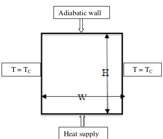
1.5 Scope
Project scope is only subjected to laminar air flow in a 2D square enclosure. This
assumption is somehow will help a lot in comparing experimental and numerical result
of the project. Also in the numerical analysis, steady state condition will be taken in
consideration. Out of all this natural convection heat transfer in square enclosure will be
focused on condition where heat is supply from below.
Figure 1.1 Heat transfer in square enclosure heated from below Adiabatic wall
Heat supply
CHAPTER II
LITERATURE REVIEW
2.1 Natural Convective Heat Transfer in Rectangular Cavity
Convection is an important type of heat transfer in technology and always occurs
in nature. For years, it has been an area of considerable interest in many fields of study
and research. There are two type of convection that is natural and force convection.
.
Natural convection heat transfer in an enclosed cavity has been a standard
comparison problem for checking the computational methodologies related to general
Navier-Stokes equations (Saitoh and Hirose, 1989). A rectangular shape would be a
simple choice in simulating the problem since square shape did not have much vary in
dimension, boundaries, and other properties related to it (Giri, et al. 2003). The
condition for a benchmark numerical solution for a square cavity is considered as wall
heated on the left side, wall cooled on the right side, and with adiabatic or perfectly
conducting boundary conditions on the upper and lower walls (De Vahl, 1983).
In a different study to create bench mark solutions to natural convection in square
cavity problems (Saitoh and Hirose, 1989), the Rayleigh number is varied while the
12
1x10⁴ and 1x10⁶ was presented. The observation can be used to validate an existing
numerical model.
In this project, simulation for basic enclodure cavity will be done first before
move to boudaries where heated from below.
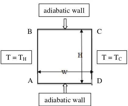
2.2 Problem Physics and Boundary Condition for Square Cavity
The physical cavity is present in Figure 2.1. temperature gradient of the cavity
will effect the generation of bouyancy. Resulting from that, the natural convection will
happen where heat transfer from wall to another in certain streamline and isotherm line.
Adiabatic wall is for controlling factor since it happen to be block all other heat or
different kind of energy from outside that can affect the result.
Figure 2.1 Problem physics and boundary condition for rectangular cavity adiabatic wall
adiabatic wall
T = TH T = TC
A
B C
13
2.3 Governing Equations for Convective Heat Transfer
In order to predict convective heat transfer rates, the distribution through the
flow field for pressure, velocity vector and temperature must be determined. Once the
distributions of these quantities are determined, the variation of any other quantity can
be obtained.
The distribution of these variables can be obtained by applying principles of
conservation of mass, conservation of momentum (Newton’s Law) and conservation of
energy (First Law of Thermodynamics). These equations for steady laminar
two-dimensional convective flow are given as follows (Cengel, 2003):
Continuity Equation :
+ = 0
Momentum Equation in x-direction :
+ = −1 + +
Momentum Equation in y-direction :
14
Energy Equation:
+ = +
2.4 Boussinesq Approximation
As discussed before, effect of temperature gradient will make changes in density
of fluid. The changes then will affect the natural convection flows in the cavity. Since
density is one of the properties of fluid, thus other fluid’s properties that vary with the
temperature effect must be take into consideration to obtain good desired result of
analysis.
The only effect on the fluid is the generation of the buoyancy terms. Density
effect in most free convective flow is relatively small and the buoyancy is the only effect
left. It cause other properties that vary with the temperature gradient will all be neglected
along with density.
1 ≤ ∆