DOI: 10.12928/TELKOMNIKA.v15i1.3854 430
Research on Topology Control in WSNs Based on
Complex Network Model
Wang Chuan-yun1,Yin Yan2 1
School of Information Engineering, East China Jiaotong University, 330013, China
2School of Software, East China Jiaotong University, 330013, China
Corresponding author, e-mail:
Abstract
A topology control algorithm based on mutual selection mechanism is proposed, combined with complex network model. It adopts node strength and spacing between nodes as the measuring parameters, selects the cluster head nodes based on mutual selection mechanism in the communication radius of nodes and builds the hierarchical topology. The algorithm can improve the clustering efficiency, shorten the average path length and save the energy of the nodes. The simulation and analysis of network evolving process and algorithm model are completed using MATLAB tools and the results verify the correctness and stability of the proposed algorithm model. The algorithm is suitable for large-scale node deployment in WSNs.
Keywords: complex network, mutual selection, wireless sensor networks, large-scale
Copyright © 2017 Universitas Ahmad Dahlan. All rights reserved.
1. Introduction
In wireless sensor networks (WSNs), network topology is the decisive factor that affects the performances of network operation efficiency and energy consumption [1], because that the sensor nodes are small devices with small batteries and recharging of these batteries is impractical in deployed scenarios. Therefore, saving energy to enhance the network’s lifetime is a main design objective in WSN [2-5]. Cluster based routing protocols decreases network complexity and give better routing efficiency [5].
But, how to achieve the clustering structure with low path length and low energy consumption is the one of the technology research hotspot in WSNs. Many research works about network topology controll methods of WSNs have been presented, and it also finds that the hierarchical topology structure has good performance. As the WSN is featured by large amounts of sensor nodes, especially in the large scale applications, complicated network structure, in this work WSN topology is analyzed on the perspective of complex network in order to build the hierarchical topology structure, shorten the path length, reduce the energy consumption and provide reference for topology optimization.
Complex network models are mainly composed by the small world network model and scale-free network model. Many researchers apply the small world theory into the study of WSNs [6-9]. In [10], the results verify that the topology of wireless sensor network is neither regular nor random, it is between random network and small-world network which has comparatively smaller average path length and bigger cluster coefficient. So the small world network model cannot be used to analyze the dynamic evolution of WSNs completely. In other words, a scale-free topology is helpful to a WSN’s performance, from the aspects of both robustness and energy efficiency. Because of such benefits, the BA model, proposed by A. L. Barabsi and R. Albert [11], has been applied in WSNs [12, 13], and a series of improvements and amendments have been made by researchers. An energy-aware evolution model for WSNs is proposed in [14]. Two topology evolution models based on BA scale-free networks are proposed, the simulation results show that the generated network topologies are robust against random and deliberate attacks [15], and in [16], an energy-aware BA model is proposed for balancing connectivity and energy consumption in WSNs.
as the measuring parameters for building the hierarchical topology structure, which can improve the clustering efficiency, balance the network load and reduce energy consumption for WSNs.
2. BA Network Evolution Model
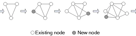
BA model is an algorithm for generating random scale-free networks using a preferential attachment mechanism. The BA network model has two basic rules: growth and preferential attachment, and preferential attachment is the key factor. Growth means that the number of nodes in the network increases over time, and preferential attachment means that the more connected a node is, the more likely it is to receive new links. Nodes with high degree have stronger ability to grab links added to the network. The evolution process of the BA model is shown in Figure 1. The new nodes are chosen by a linear preferential attachment rule, i.e. as shown in formula (1), the probability of the new nodes to connect with an existing node j is proportional to the degree of j,
∑
(1)
Therefore, the most intimately connected nodes have greater probability to receive new nodes, known as “the rich get richer” paradigm.
Existing node New node
Figure 1. Evolution Model of BA Scale-Free Network
3. The WSNs Topology Control Algorithm Based on Mutual-selection Mechanism 3.1. Related Definitions
1) Node strength (S)
In a weighted network of N*N, wij is the weight of edge (i, j),i, j=1, 2...N. Si can be denoted by formula (2).
∑ (2)
Where
(
i
)
is a set of all the nodes connected to the node i, and S is the strength threshold of all nodes, Si ≤ S. Additionally, it only considers the undirected network in this paper, so wij=wji. In WSNs, wij represents the traffic between nodes i and j, and Si represents the traffic through node i.2) Average shortest path length(L)
The average distance of a network is defined as the average value of all distances over the network, defined as formula (3):
∑ (3)
Where dij, the distance between node i and j, indicates the total number of edges between node i and j in the shortest path.
3) Average clustering coefficient(C)
The ratio between the real and the possible number of edges in the cluster of the ki nodes is defined as the clustering coefficient of node i, denoted as Ci ; namely:
Where ki is neighbors of node i, ei is the number of the actual edges existing among the ki nodes. Then, the average clustering coefficient, denoted as C, represents the average of all clustering coefficients in the network given by:
∑ (5)
4) Energy consumption
Energy consumption is proportional to the data transmission distance. The distance threshold d0 is defined as formula (6) [17].
√
(6)
Where Efs and Eamp represent the energy required to power amplification in free space channel model and multipath fading channel model respectively. According to formula (7) and (8), we can get the energy consumption when d< d0 and d> d0 respectively in free-space channel model and multipath fading channel model.
{ (7)
(8)
Where Eelec and denotes the energy consumption per bit of data for transmitting or receiving and power amplification loss coefficient respectively, and k indicates the number of bits transmitted or received.
3.2. Process of Algorithm Model
On the basis of the BA model in this paper, we adopted mutual-selection mechanism, using node strength as key parameter, to build the hierarchical topology structure for WSNs. In the whole process of the algorithm, we assumed that all sensor nodes are identical and stationary after deployment, each node has a unique coordinate.
1) Initialization: the network begins with an initial connected network of m0 nodes. The initial weight value of each edge between two nodes is w0.
2) Network growth: new nodes are added to the existing network one at a time and introducing links to m(m≤m0) existing nodes with preferential attachment so that the probability of linking to a given node i is proportional to the number of existing links Si that existing nodes have, i.e.,
∑ (9)
Remark: the weight each new edge is also set to w0. 3) Mutual selection
(1) Start from base station: selecting the nearest node i with the maximum Si from the base station as the highest level cluster head. And then, the cluster head nodes in level K are determined in turn (the value of K is determined by the size of network), i.e.: the cluster head node i in the higher layer select candidate head node j of next level from its neighbor nodes located in its communication radius R.
(2) Mutual selection: according to formula (10), the connection building between nodes i and j is due to fij. If a pair of unlinked node i and j is mutually selected, i.e.: if fij or fji is the maximum value and then a connection will be built between nodes i and j.
(10)
√ (11)
4) Clustering: each cluster head nodes broadcast its ID to the other neighbor nodes which include the cluster head nodes and the common nodes, then, the common nodes select the nearest cluster head node in the communication radius for building the connection, and finally, the clusters are formed.
Remark: if the strength of cluster head node i meet the equation:Si>S,then the evolution process goes back to step 4).
5) If some nodes are not in any clusters due to the communication radius, these nodes will join the nearest cluster.
3.3. Dynamic Evolution
1) Process of weight evolution
More specifically, the newly added link to node i have a larger impact on the node i than the far ones. For analyzing easily, the influence region of node i is set as direct neighborhood of node j.
Where represents that the newly added edge brings additional traffic burden to edge (i, j). 2) Analysis of node strength
The network starts from an initial connected network of m0 nodes and grows with new node added one at a time till the total node number reached N. Hence, the evolution time of the model is equivalent to the number of nodes added to the network, i.e., t=N-m0, and the natural time scale of the model is the network size N. Using the continuous approximation, so we can regard the edge weight w, the node strength S and the time t as continuous variables. And then, the edge weight wij is updated according to evolution equation (14):
∑ ∑ (14)
There are two processes that contribute to the increment of strength Si. One is the creation of connection with node i, the other is the attachment to node i by newly added node. So, the rate equation of strength Si can be written as below:
which can be easily integrated with initial conditions Si(t=i)=n,this yields:
Thus, the knowledge of the time evolution of the variables permits us to compute their statistical properties. Actually, the time ti=t at which the node i enters the network is uniformly distributed in [0, t] and the strength probability distribution can be given as:
∫ (18)
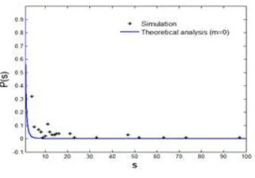
Where is the Dirac delta function. Using the equation Si~(t/i)θ obtained from formula (17), we obtain the strength distribution P(s)~S-α with α=1+1/θ in the infinite size limit .
[ ] [ ] (19)
Obviously, when m=0 the model is recovered to the BA network and the value α=3.
4. Simulation and Analysis
We use MATLAB to simulate the wireless sensor network and analyze the performance of the algorithm. The relative parameters are shown in Table 1. The network evolution result with the time is shown in Figure 2. And then, the relative simulation analysis is performed in the Figure 3.
Table 1. The Set Value of Parameters
Parameters Value
Size 100m*100m
R 50m
m0 8
M 2
w0 2
Figure 2. Network Evolution Model based on BA Model Algorithm
Figure 3 shows the distribution of the strength S, the simulation consistency of scale-free properties indicates that our model can indeed produce power-law distributions of the strength S. In this case, the simulation of the model reproduces the behaviors predicted by the theoretical analysis.
Figure 4 shows the changing trend of average clustering coefficient C with the growth of nodes. In the simulation setting, we change the value of the parameters as m0=5,m=2; m0=5,m=3; m0=8,m=2 and m0=8,m=3 for the proposed model. Numerical simulations indicate that the changing trends of the average clustering coefficient C are gentle, in line with the shifting trend of the strength S, and the C values are nearly stable with the increase of the network size,and also from Figure 4, we can get the result that the value of C raises with increasing the number of connected nodes for new added nodes in the process of network growth, which corresponds with the real networks.
Figure 4. Evolution of C
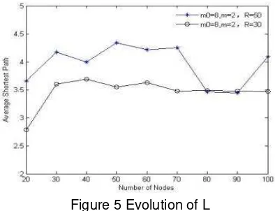
Figure 5 gives the comparison of the average shortest path as R=30 and R=50 with the growth of network. From Figure 5, we find that the value of the average shortest path length is smaller and has the gentle change trend, which verifies the stability and the lower energy consumption of the proposed model.
Figure 5 Evolution of L
Figure 6. Topology Structure based on MSM
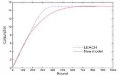
As shown in Figure 7, we make the comparison with the classic LEACH algorithm which is one of the preliminary research fields in WSNs application of our group. The energy consumption curve of new model(MSM) is more smooth and curved than classic LEACH algorithm. Because that energy consumption is proportional to the data transmission distance according to formula (7). In the new model based on MSM, the distribution of cluster heads in the network is uniform, the distance between cluster head nodes and normal nodes are almost in the range of the threshold, so the energy consumption of the network is more evenly. But LEACH algorithm does not guarantee a uniform distribution of cluster heads in a network, which may result the most of the transmission distance out of range of the threshold and so increasing the energy consumption of the network.
Figure 7. Comparison of Energy Consumption
5 Conclusion
Acknowledgements
This research program is supported by National Natural Science Foundation of China (61462028), Science and Technology Support Plan of Jiangxi province, China (20151BBE50097), and Science and Technology Project of Educational Department in Jiangxi Province (GJJ150545).
References
[1] ME Haque, MFM Zain, M Jamil. Performance Assessment of tree topology sensor network based on scheduling algorithm for overseeing high-rise building structural health information. International Journal for Light and Electron Optics. 2015; 126(18): 1676-1682.
[2] Khalid Haseeb, Kamalrulnizam Abu Bakar, Abdul Hanan Abdullah, et al. Improved Energy Aware Cluster based Data Routing Scheme for WSN. TELKOMNIKA. 2016; 14(2): 531-537.
[3] Vaibhav Godbole. Performance Analysis of Clustering Protocol using Fuzzy Logic for Wireless Sensor Network. IAES International Journal of Artificial Intelligence. 2012; 1(3): 103-111.
[4] Rony Teguh, Hajime Igarashi. Optimization of Sensor Network Topology in Deployed in Inhomogeneous Lossy Media. TELKOMNIKA. 2015; 13(2): 469-477.
[5] Khalid Haseeb, Kamalrulnizam Abu Bakar, Abdul Hanan Abdullah et al. Grid Based Cluster Head Selection Mechanism for Wireless Sensor Network. TELKOMNIKA. 2015; 13(1): 269-276.
[6] Zheng Gengzhong, Liu Qiumei. A Survey of Wireless Sensor Networks Based on Small World Network Model. International Conference on Electrical and Control Engineering. 2010: 2647-2650. [7] Dong Wang, Erwu Liu, Zhengqing Zhang, et al. A Flow-Weighted Scale-Free Topology for Wireless
Sensor Networks. IEEE COMMUNICATIONS LETTERS. 2015; 19(2): 235-238.
[8] Helmy A. Small worlds in wireless networks. IEEE Communication Letters. 2007; 7(10): 490-492. [9] Gaurav Sharma, Ravimazumdar. Hybrid Sensor Networks. A Small World, ACM MOBIHOC. New
York: ACM Press. 2009: 366-377.
[10] Ren Yueqing, Xu Lixin. Study on Topological Characteristics of Wireless Sensor Network Based on Complex Network. 2010 International Conference on Computer Application and System Modeling. 2010; 15: 486-489.
[11] AL Barabsi, R Albert, Emergence of scaling in random networks. Science. 1999; 286(5439): 509-512. [12] Shizuka M, Masaki A. The reliability performance of wireless sensor networks configured by
power-law and other forms of stochastic node placement. IEICE transactions on communications. 2004; 87(9): 2511-2520.
[13] M Enachescu, A Goel, R Govindan, R Motwani. Scale free aggregation in sensor networks. In Algorithmic Aspects of Wireless Sensor Networks. Berlin, Germany: Springer-Verlag. 2004: 71-84. [14] Zhu H, Luo H, Peng H, et al. Complex networks-based energy-efficient evolution model for wireless
sensor networks. Chaos, Solitons & Fractals. 2009; 41(4): 1828-1835.
[15] Zheng G, Liu S, Qi X. Scale-free topology evolution for wireless sensor networks with reconstruction mechanism. Computers & Electrical Engineering. 2012; 38(3): 643-651.
[16] Y Jian, E Liu, Y Wang, Z Zhang, C Lin. Scale-free model for wireless sensor networks. In Proc. IEEE WCNC. 2013: 2329-2332.