2D ELASTICITY ANALYSIS
WITH BOUNDARY ELEMENT METHOD
Supriyono
Departement of Mechanical Engineering, Faculty of Engineering, Muhammadiyah University of Surakarta.
Email: [email protected]
ABSTRACT
In this paper, a boundary element method for 2D elasticity analysis is presented. The formulations are also presented. Numerical integration is applied to solve the boundary integral equation obtained from the formulation. Quadratic isoparametric elements are used to represent the variation of a variable along an element. Several examples are presented to demonstrate the validity and the accuracy of the method.
Keywords: elasticity-numerical integration-isoparametric element-boundary element method.
Introduction
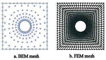
In general, there are three popular numerical methods used in practical problems, the Finite Difference Method (FDM), the Finite Element Method (FEM) and the Boundary Element Method (BEM). FDM and FEM are called domain methods as the discretization of the domain is required. On the other hand, the BEM (Brebbia, 1984) is known as a boundary type method. The most interesting feature of the Boundary Element Method (BEM) is that only the boundary of the model needs to be discretized, thus the dimensionality of the problem is reduced by one. It means that for two-dimensional problems, only the line-boundary of the domain needs to be discretized into elements, and for three-dimensional problems only the surface of the problem need to be discretized (see Fig. 1). Further advantages can be found in the continuous modelling of the interior and usually a coarser discretization is needed compared to Finite Element Method meshes. The BEM’s applicability at present is not as wide ranging as FEM, however the method has become established as an effective alternative to
FEM in several important areas of engineering analysis.
Figure 1. BEM vs FEM mesh in 2D
of the physical parameters can be obtained by simple integrations.
The fundamentals of the BEM can be traced back to classical mathematical formu-lations by Betti (1872), Somigliana (1886), Fredholm (1903), and Mikhilin (1957), The works by Fredholm and Mikhilin were for potential problems, whereas the works of Betti and Somigliana dealt with elasticity problems. The development of the formulations in the context of boundary integral equation is due to Jaswon (1963), Massonnet (1965), Hess and Smith (1967), Rizzo (1967) and Cruse (1969). Cruse was the first one who introduced three-dimensional elastostatics in boundary element method. The work of Lachat and Watson (1976) is perhaps the most significant early contribution towards BEM becoming an effective numerical technique. They developed an isoparametric formulation similar to those used in the FEM and demonstrated that BEM can be used as an effective tool for solving problems with complex configuration. Since these early contributions of the BEM, much progress has been made in many different applications. Several authors have written text books on BEM, such as Aliabadi (2001), Brebbia (1992), Banerjee(1992), Becker (Becker1992), and Wrobel (2001).
This paper presents the application of BEM to two dimensional (2D) elastostatic problems. Throughout this paper, the cartesian tensor notation is used, with the Latin indices varying from 1 to 2.
Displacement and Stress Integral Equations
Applications BEM in solid mechanics are based on the Somigliana’s identities. Somigliana’s identity for displacements in 2D elasticity problems
states that the displacements at any points X’
[ui(X’)] belonging to domain (X’ЄV) to the boundary values of displacement [uj(x)] and traction [tj(x)] can be expressed as (Aliabadi, 2001):
fundamental solutions representing a
displace-ment and a traction in the j direction at point x due to a unit point force in the i direction at point
X’. These fundamental solutions can be found in
Aliabadi (2001).
Equation (1) is valid for any source points within domain (X’ЄV), in order to find solutions on the boundary points, it is necessary to consider the limiting process as X’→x’ S. The limiting process can be found in many text book, for examples Aliabadi (2001), Brebbia (1992), Banerjee(1992), Becker (Becker1992), and Wrobel (2001). After limiting process, boundary displacement integral equations can be expressed as
The Somigliana’s identity for stresses can be expressed as
fundamental solutions and can be found in the same text book as mentioned above.
As equation (1), equation (3) is valid for any source points within domain (X’ЄV), to find stresses on the boundary, two methods are
available. The first commonly called as indirect
approach relies on using recovered boundary
tractions and displacements obtained from the BEM solutions using equation (2). The tangential strains are calculated by differentiation of equation (2) and then the strains are converted by Hooke’s law and Cauchy’s formula to have
the stresses. The second method is called direct
approach. The stresses can be obtain by limiting
process of equation (3) as X’→x’ S. This
Dicretization and System of Equation
In order to solve equation (2), a numerical method is implemented as analitic solution is almost impossible due to complexity of the equation. The boundary S is discretized into Ne using quadratic isoparametric elements as can be seen in Figure 2.
Figure 2. Discretization
In this formulation, boundary parameter
xj, the unknown boundary values of
dis-placements ujand tractions tj are approximated using interpolation function, in following manner:
∑
The shape functions Ná are defined as
)
Substituting equation (4) and equation (5) into equation (2), one gets (the integrations on the boundary S): daries S and Jn is the Jacobian transformations.
After discretization and point collocation on the boundary the equations (6) can be written in the matrix form as
[ ]
H{ }
u =[ ]
G{}
t (7)where [H] and [G] are the well-known boundary element influence matrices. {u}, {t}, are the dis-placement and the traction rate vectors on the boundary.
After imposing boundary condition, equations (7) can be written as
[ ]
A{ } { }
x = f (8)where, [A] is the system matrix, {x} is the
unknown vector and {f } is the vector of
prescribed boundary values.
In similar way, the stress integral equations of equations (3) can be presented in matrix form as
[ ] [ ]
σ = G{ }
t −[ ]
H{ }
u (9)At this point, it can be seen that the stresses at internal points are calculated using equation (9) after the boundary values of displacements and tractions are found from equation (8).
Examples
In order to show the accuracy and the validity of the method presented above, examples are shown as follows:
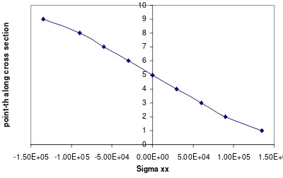
Figure 3. Distribution of normal stress along the cross section of cantilever beam
0
Figure 4. Distribution of shear stress along the cross section of cantilever beam
0 1 2 3 4 5 6 7 8 9 10
0.00E+00 2.00E+03 4.00E+03 6.00E+03 8.00E+03 1.00E+04 1.20E+04 1.40E+04 1.60E+04
Sigma xy
p
o
in
t-th
a
lo
n
g
c
ro
s
s
se
c
ti
o
n
Conclusion
Some points can be drawn from the pre-sentation above:
1. The most interesting feature of BEM is reducing dimensionality of the problem by one.
REFERENCES
Aliabadi, M.H., The Boundary Element Method, vol II: application to solids and structures, Chichester, Wiley (2001).
Banerjee, P.K., The Boundary Element Method in Engineering, McGraw-Hill, New York (1992).
Becker, A., The Boundary Element Method in Engineering, McGraw-Hill, London (1992).
Betti, E., Teoria dell’elasticita’, Il Nuovo Cimento, 7-10, (1872).
Brebbia, C.A., Dominguez, J., Boundary Elements, an Introductory Course, 2nd edition, Computational Mechanics Publication, Southampton, McGraw-Hill Book Company, New York, (1992).
Cruse, T.A., Numerical solutions in three-dimensional elastostatics, International Journal of Solids and Structures, 5, 1259-1275, (1969).
Fredholm, I., Sur une classe d’equatios fonctionelles, Acta Mathematica, 27, 365-390, (1903).
Hess, J.L., and Smith, A.M.O., calculation of potential flows about arbiratry bodies, Progress in Aeronautical Sciences, 8, Perganon Press, (1967).
Jaswon, M.A., Integral equation method in potential theory, I, Proceeding of the Royal Society of London, Series A, 275, 23-32, (1963).
Lachat, J.C., Watson, J.O., Effective numerical treatment of boundary integral equations, International Journal for Numerical Methods in Engineering, 10, pp.991-1005, (1976).
0.00E+00 5.00E+03 1.00E+04 1.50E+04 2.00E+04 2.50E+04 3.00E+04
0 2 4 6 8 10
Point-th arround the hole
Si
g
m
a vo
n
M
ises
Cir-Ex Fully Modelled NE.GT.1st one Smaller diameter larger diameter
Figure 5. Stress distribution of circular excavation plate due to tension (The points was taken in the y direction
along side the diameter of the hole)
2. The discretization technique of BEM is the same as FEM discretization.
Massonnet, C.E., Numerical use of integral procedure, In Stress Analisys, Chapter 10, 198-235, Wiley, London, (1965).
Mikhilin, S.G., Integral Equation, Pergamon Press, London, (1957).
Rizzo, F.J., An integral equation approach to boundary-value problems of classical elastostatics, Quarterly Journal of Applied Mathematics, 25, 83-95, (1967).
Somigliana, C., Sopra l’equilibrio di un corpo elastico isotropo, Il Nuovo Cimento, serie III, vol.20, 81-185,(1886).