METHODOLOGY AN APPROPRIATE LOT SIZING TECHNIQUE FOR INVENTORY POLICY PROBLEM WITH DECREASING DEMAND.

(1)

11 CHAPTER 3

METHODOLOGY

The research in this thesis focuses on finding an appropriate lot sizing technique

in decreasing demand problem that gives minimum total cost. This chapter

explains about the methodology used by the researher to do the research. The

methodology is started from problem identification, literature review, research

preparation, generating 2 solution models, result analysis, and conclusion. Those

are explained as follows:

3.1. Problem Identification

This was the first step taken by the author to identify the problem of the research.

The author was using the decreasing demand problem happened in hard drive

manufacturer as the example problem. There were 5 items of HGA (Head Gimbal

Assembly) those were assembled by 2 components. There were suspension and

slider fabrication. The author focused on suspension component rather than

slider fabrication because this component should be bought by the company from

suppliers. Materials Department – Suspension Commodity was the department who took the responsibility to buy the suspension. They faced a problem to

minimize the total cost from over-buying suspensions. This step was explained in

Chapter 1 of this research.

3.2. Literature Review

After identifying the problem of the research, the next step was conducting

literature review. This step was conducting by the author to find the possible

research in decreasing demand problem. Author had reviewed some papers

related to decreasing demand problem, but just a few papers conducting Lot

Sizing Technique to solve the problem. One paper from Pujawan and Kingsman

(2003) was used as a guideline to do this research. Their paper explained about

the properties of lot sizing technique for Lumpy Demand. They conducted 5

different Lot Sizing techniques on his research: Silver Meal 1(SM1); Silver Meal2

(SM2); Least Unit Cost (LUC); Part Period Balancing (PPB); and Incremental

(ICR) techniques. They suggested an appropriate lot sizing technique to

minimize total cost for Lumpy Demand problem. Author found the gap to conduct

(2)

This step was explained in Chapter 2 and added theoretical background of Lot

Sizing technique. Figure 2.1 showed the gap analysis of this research.

3.3. Model Development

This step was conducted by the author to make some preparations before

conducting the research. First, author checked the data distribution whether it

followed the decreasing demand characteristic or not. The data followed

decreasing demand pattern and exponentially distributed. Those were explained

in Chapter 4. Second, author constructed 2 solution models for the research

problem. Considering the research was about inventory policy problem with

dependent demand characteristic, author conducted different treatments to

parents(HGA) and components(Suspension) of items in order to see the effect in

calculating total cost. There were explained as follow:

a) Solution model 1:

Author constructed MRP sheet in excel for 5 lot sizing techniques. The parent’s quantity orders were solved by using Lot For Lot technique and the components were solved by using 5 lot sizing techniques: Silver Meal 1,

Silver Meal 2, Least Unit Cost, Part Period Balancing, and Incremental. Then,

author calculated the Total Cost for each item per lot sizing technique.

b) Solution model 2:

Author constructed MRP sheet in excel for 5 lot sizing techniques. The parent’s and component quantity orders were solved by using 5 lot sizing techniques: Silver Meal 1, Silver Meal 2, Least Unit Cost, Part Period

Balancing, and Incremental. Then, author calculated the Total Cost for each

(3)

[image:3.595.92.505.97.423.2]

13

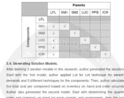
Table 3.1. The pairs of Lot Sizing Technique

Parents

LFL SM1 SM2 LUC PPB ICR

C

ompo

ne

nts

LFL

SM1 √ √

SM2 √ √

LUC _√ √

PPB _√ √

ICR _√ √

3.4. Generating Solution Models.

After defining 2 solution models in this research, author generated the solutions.

Start with the first model, author applied Lot for Lot technique for parent’s demands and 5 different techniques for the components. Then, author calculated

the total cost per component based on inventory on hand and order occurred.

Author also generated the second model. Start with determining the quantity

order and inventory on hand for each parents and components, then the total

cost for each component was calculated. This step was explained in Chapter 5

and Chapter 6.

3.5. Result Analysis

This step was intended to compare the results of each model used. Author

compared the total cost occurred from different lot sizing techniques. Total cost

occurred from inventory cost and order cost. The results of these calculations

were calculated by using simple calculation in Microsoft© Excel 2007. The aim of

comparing the results between first and second solution model was to find what

kind of lot sizing technique can be used in decreasing demand problem to

minimize total cost. The result analysis is discussed in Chapter 7 of this research.

3.6. Conclusion

The results from analytical model calculation and analysis were used in taking the

conclusion. This step was intended to check if the objective of the research had

been achieved. The conclusion of this research is presented in Chapter 8. The

(4)

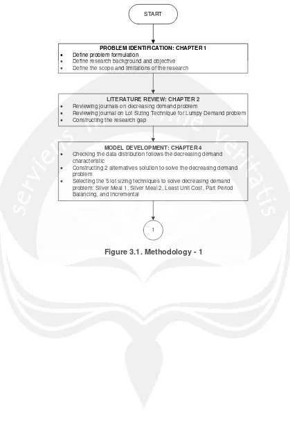
START

LITERATURE REVIEW: CHAPTER 2 · Reviewing journals on decreasing demand problem

· Reviewing journal on Lot Sizing Technique for Lumpy Demand problem · Constructing the research gap

PROBLEM IDENTIFICATION: CHAPTER 1 · Define problem formulation

· Define research background and objective · Define the scope and limitations of the research

MODEL DEVELOPMENT: CHAPTER 4 · Checking the data distribution follows the decreasing demand

characteristic

· Constructing 2 alternatives solution to solve the decreasing demand problem

· Selecting the 5 lot sizing techniques to solve decreasing demand problem: Silver Meal 1, Silver Meal 2, Least Unit Cost, Part Period Balancing, and Incremental

[image:4.595.90.509.80.706.2]

1

(5)

15

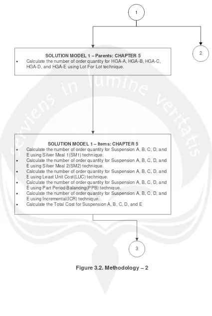
SOLUTION MODEL 1 – Parents: CHAPTER 5

· Calculate the number of order quantity for HGA-A, HGA-B, HGA-C, HGA-D, and HGA-E using Lot For Lot technique.

SOLUTION MODEL 1 – Items: CHAPTER 5

· Calculate the number of order quantity for Suspension A, B, C, D, and E using Silver Meal 1(SM1) technique.

· Calculate the number of order quantity for Suspension A, B, C, D, and E using Least Unit Cost(LUC) technique.

· Calculate the number of order quantity for Suspension A, B, C, D, and E using Part Period Balancing(PPB) technique.

· Calculate the number of order quantity for Suspension A, B, C, D, and E using Incremental(ICR) technique.

· Calculate the Total Cost for Suspension A, B, C, D, and E 1

3

[image:5.595.87.512.78.712.2]

2

(6)

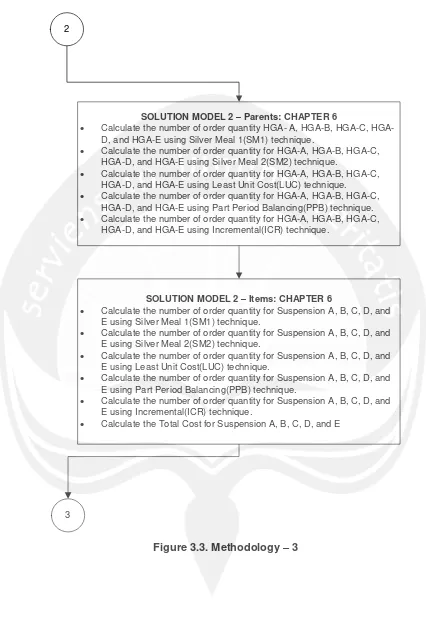
SOLUTION MODEL 2 – Parents: CHAPTER 6

· Calculate the number of order quantity A, B, C, HGA-D, and HGA-E using Silver Meal 1(SM1) technique.

· Calculate the number of order quantity for HGA-A, HGA-B, HGA-C, HGA-D, and HGA-E using Silver Meal 2(SM2) technique.

· Calculate the number of order quantity for HGA-A, HGA-B, HGA-C, HGA-D, and HGA-E using Least Unit Cost(LUC) technique.

· Calculate the number of order quantity for HGA-A, HGA-B, HGA-C, HGA-D, and HGA-E using Part Period Balancing(PPB) technique. · Calculate the number of order quantity for HGA-A, HGA-B, HGA-C,

HGA-D, and HGA-E using Incremental(ICR) technique.

SOLUTION MODEL 2 – Items: CHAPTER 6

· Calculate the number of order quantity for Suspension A, B, C, D, and E using Least Unit Cost(LUC) technique.

· Calculate the number of order quantity for Suspension A, B, C, D, and E using Part Period Balancing(PPB) technique.

· Calculate the number of order quantity for Suspension A, B, C, D, and E using Incremental(ICR) technique.

· Calculate the Total Cost for Suspension A, B, C, D, and E

[image:6.595.86.512.74.703.2]

3 2

(7)

17

RESULT ANALYSIS: CHAPTER 7

· Comparing the result from analytical model calculation with different Alternative solutions, in order to check the appropriate lot sizing method for decreasing demand problem

CONCLUSION: CHAPTER 8

[image:7.595.88.510.68.724.2]

END 3