JOURNAL OF
SOUND AND
VIBRATION
Journal of Sound and Vibration 310 (2008) 287–312
Continuous-time covariance approaches for modal analysis
Giuseppe Quaranta
, Pierangelo Masarati, Paolo Mantegazza
Dipartimento di Ingegneria Aerospaziale, Politecnico di Milano via La Masa, 34 20156 Milano, Italy
Received 25 July 2006; received in revised form 11 May 2007; accepted 30 July 2007 Available online 24 October 2007
Abstract
Proper orthogonal decomposition (POD) can be used to obtain complete information about the linear normal modes of structural systems only when special conditions are met, principally related to the knowledge of mass distribution and to the absence of damping. The main advantage of POD is the possibility to directly use covariance matrices estimated from time responses for the modal identification of the structure under investigation. This paper proposes a method to extend this covariance-based identification to general cases where significant damping is present and when no data is available on mass distribution. A least-square based decomposition is used to infer information about modal characteristics of the system. This decomposition is applied to three different cases: the first one uses records related to the free response of the system, while the remaining two use records of the system under persistent white noise excitations. In those latter cases the information on the excitation input time history can either be used, or treated as unknown. Basic, yet complete examples are presented to illustrate the properties of the proposed technique.
r2007 Elsevier Ltd. All rights reserved.
1. Introduction
The proper orthogonal decomposition (POD) is a powerful method, based on singular value decomposition (SVD), that is widely adopted to capture the dominant signals from the analysis of multidimensional time series. It has been applied, often with different denominations such as Karhunen–Loe`ve Decomposition, in many branches of engineering, either for linear or nonlinear systems. For a good survey of the related literature, and for details on implementations and applications, the reader should refer to the work of Kershen et al. [1]. This technique has a much longer tradition in statistics, where is known as principal component analysis (PCA), aimed at the reduction of dimensionality in multivariate data set with the determination of a new set of variables which retains most of thevariationpresent in the original set[2]. The first descriptions of the PCA can be traced back to the work of Pearson[3]in 1901 and Hotelling[4]in 1933. It can be easily shown that the optimal set of dimensionnis composed by the firstneigenvectors of the covariance matrix ordered in terms of the magnitude of the related eigenvalues, which correspond to the first n singular vectors of the observation matrix composed by themcolumn vectors of thepmeasures.
www.elsevier.com/locate/jsvi
0022-460X/$ - see front matterr2007 Elsevier Ltd. All rights reserved. doi:10.1016/j.jsv.2007.07.078
Corresponding author. Tel.: +39 0223998362.
Usually, POD analysis is applied to matrices describing the covariance of variables measured at the same time[1]. Other authors (e.g. Ref.[5]), compute covariance matrices of unsteady phenomena in the space of the samples, called ensemble, instead of in time. In any case, the dynamic relationship between consecutive samples in time, that the variables under investigation possess, appears to be not sufficiently taken into account by the POD, as it should. The reason is that POD does not explicitly take into account the cross-covariance between a measure and its derivative, assuming that both are available, to account for the dependency on the time shift between the measured variables[6].
In the structural dynamics field, special efforts have been dedicated to finding a physical interpretation for the POD modes[7–9]. Significant research effort has been dedicated to finding a correlation between the POD and the linear normal modes, which represent a more ‘‘classical’’ set of basic forms used for the dimensional reduction of dynamic structural systems, with the aim of using the POD as a modal analysis tool [9]. For undamped systems, Feeny and Kappagantu[7]showed that proper orthogonal modes (POMs) converge to the normal modes in free vibration analysis. The same holds true when random, white noise excitation is used
[8,9]. However, in Ref.[9]it is stated that nothing can be said on the value of the frequency related to each mode if the mass distribution of the system is not known. As a consequence, additional frequency domain analysis of the POMs time series is required for the extraction of the related information[10–12]. Feeny and Kappagantu[7]formulated a hypothesis on the possible use of the derivatives of the state measures to solve the problem when damped systems are under investigation, but they did not pursue this research line. In order to recover the information on the frequency, Chelidze and Zhou [13] introduced what they called smooth orthogonal decomposition (SOD), which uses a numerically approximated covariance matrix of the derivatives of the measures, together with the usual covariance of the measures, to obtain additional information. However, this method suffers from the limitation of being exactly applicable only to undamped systems, and only provides an estimate of the frequency as the sample time increases.
To overcome all these problems, and to derive a more general method to recover the information on the dynamic characteristics of the system under investigation using covariance matrices, another method is here introduced. This method originates from the simple observation that least squares can be used to extract the eigenvalues and eigenvectors of a mechanical system from its time response. The proposed methodology works for generally damped systems and allows the identification of modal forms with the related eigenvalues without any prior knowledge of the mass distribution. The possibility to identify damped systems is extremely important when structures, like aircraft, interacting with the surrounding fluid, are investigated. The crucial piece of information, neglected by other authors in previous works, is the cross-covariance matrix between the measures and their derivatives, as shown in Section 2. Of course, this means that the measure derivatives must be either acquired, or somehow restored from the known data using a finite difference numerical operator, as in Ref.[13]. In any case, since the numerical differentiation is known to introduce additional noise in the signals, an integral numerical operator can be used, which acts as a filter instead. In this case, the role of the basic signals is played by the integrated ones, while the measured signals act as their derivatives.
Section 2 presents the basic idea introducing a new orthogonal decomposition of the data which could be denominatedproper dynamic decomposition(PDD), since it started as an extension of the POD methods taking into account the fact that the time series under analysis are observations of a dynamic system data. Section 3 gives an interpretation of the obtained modes when free responses are used as time histories, which directly allows to recover the normal modes of the system, together with the associated frequency and damping values. Section 4 gives an interpretation for the case of responses obtained from persistent excitations, which again allows to recover the normal modes, with the associated frequency and damping. The last two sections are completed by simple examples, both analytical and numerical, to illustrate the quality of the proposed method. Incidentally, what is presented results in a methodology to recover the information on the characteristics of the dynamics of the system under analysis directly by a continuous time domain approach instead of going through a preliminary discrete identification, even though this was not an objective of the work.
2. Transient response analysis
Consider a set of measuresxðtÞ 2Rm, that are functions of timet2½0;t, obtained as free responses of a
unknown vectorU2Cm
q¼xTU (1)
to yield a scalar functionqðtÞ 2C1 that satisfies the linear differential equation
_
q¼lq, (2)
wherel2Cis unknown.1
The aim of the proposed analysis is to represent the generic transient response, not limited to the free response of a dynamic system, into a set of generic modes, and thus can be viewed as a PDD. The resulting PDD, consisting in the proper dynamic modes (PDMs) U and the corresponding proper dynamic values (PDVs)l, represents a decomposition of the analyzed signals in a minimal set of damped harmonic signals of the type Uielit, which can be combined with the conjugate solution, when complex, to obtain the real
expression
xðtÞ ¼eReðliÞtðReðU
iÞcosðImðliÞtÞ þImðUiÞsinðImðliÞtÞÞ. (3)
The classification of the PDMs can be done in terms of frequency, damping or both, depending on the specific properties sought for the PDD. It is worth stressing that only the eigensolutions observable with the considered measures can be effectively recovered using this type of analysis.
In general, Eq. (2) cannot be strictly satisfied by a generic vector U, so the problem
_
xTUffilxTU (4)
yields a residual errore:
ðlxx_ÞTU¼e, (5)
which needs to be minimized to obtain an optimal vectorU. An integral measure of the overall square error over the measure interval 0½ ;tis
which can be minimized by an appropriate selection of the multipliersU:
min
U ðJÞ. (7)
The minimization with respect toU of Eq. (6) leads to
qJ
which represents a second-order eigenproblem, wherelis the eigenvalue andUis the eigenvector[14]. If either the mean value of the vector x is null, or it is removed, the matrices Rxx and Rx_x_ 2Rmm represent the
deterministic auto-covariances(often simply denominated covariances) of the state and of its time derivative, respectively (for a definition of covariances see, Ref.[15]). The adjective ‘‘deterministic’’ is added to emphasize the fact that these matrices only converge toward the ‘‘statistical’’ variances for t! 1. In this sense, as opposed to the usual meaning of ‘‘non-randomly forced’’, it was already used in Ref. [16]. However, that qualification will be dropped in the following to simplify the language, since the meaning should be clear from the context.
These covariance matrices are usually the piece of information used for the extraction of POD which is composed by the proper orthogonal values (POVs), the eigenvalues of Rxx, and the corresponding modes
1Actually, since x
2Rm, for each l2C with ImðlÞa0 there will exist conjugates l, U such that qþq;q_þq_2R1, and
(POMs)[1]. The matrixRxx_ represents thecross-covariance between the state derivative and the state itself,
while, by definition, it may be shown that Rxx_ ¼RTxx_ . The latter matrix plays a crucial role for the correct
identification of eigensolutions when significant damping is present, as shown in the following.
The resulting eigenproblem is not in general related to the system state matrix, but represents a least square approximation of the generic transient response problem into a set of complex modes (PDMs). In a fashion similar to the SOD decomposition presented in Ref.[13], this PDD is invariant with respect to any linear, non-singular coordinate transformation. In fact, if a new set of coordinatesy¼Tx is defined, Eq. (8) becomes
~
2.1. Requirements on measure availability
The proposed approach requires a set of measuresx and its time-derivatives x_. In practical applications (system identification from numerical simulation output, or from experimental measurements), different combinations of measures may be available. Typically, in case of numerical simulations, the entire state and its derivatives is available; however, when only partial information is available, the missing part needs to be estimated.
When only position measuresyare available, velocitiesy_and accelerationsy€can be computed by numerical differentiation. This is likely to yield significantly noisy derivatives, unless appropriate filtering is used. In this work, centered differences,
have been used to compute position derivatives. Centered differences have been selected to avoid phase shift in the derivatives.
When only acceleration measuresy€are available, velocitiesy_and positionsycan be computed by numerical integration. This process is expected to naturally filter out measurement noise. In this work, this second approach has not been directly used; however, non-trivial numerical problems have been usually integrated using Matlab standard integration algorithms, basically resulting in a form of numerical integration of the accelerations. Future work will address the practical application of this technique to experimental measures.
3. Free response
Consider Eq. (4) before multiplication by vectorU,
_
xffilx, (11)
where the actual system can be represented by a simple, constant coefficient autoregressive (AR) model
_
x¼Ax, (12)
withA2Rmm. In this case, Eq. (5) can be written as
ðlxAxÞTU¼e. (13)
The same minimization procedure as in Eq. (8) leads to
¼ ððlIAÞRxxðlIATÞÞU ð14Þ ¼ ðl2RxxlðARxxþRxxATÞ þARxxATÞU. ð15Þ
Considering Eq. (8), the following correspondences can be recognized:
Rxx_ ¼ARxx (16)
Rx_x_ ¼ARxxAT ¼Rxx_ AT
¼ARxx_. ð17Þ
The essential difference is that the covariance matrices of Eq. (15) result from the free response of a linear system, so they exactly contain the dynamics of matrixA, while those of Eq. (8) describe a generic transient response.
Two different estimates of matrixAcan be obtained from the covariances of a free response analysis,
A¼Rxx_ Rxx1, (18)
A¼Rx_x_Rxx_1, (19)
where Eq. (18) corresponds to the classical AR identification resulting from the application of least-squares[17].
Expression (14) highlights the fact that the previously mentioned second-order eigenproblem, in this specific case, is actually the product of problem (13) and its transpose. But, since the eigenvalues ofAand ofAT are the same[18], the eigenvalues of the second-order problem are twice those of matrixA. They can be obtained, for example, from either of the problems
ðRxx_lRxxÞx¼0, (20)
ðRx_x_lRxx_ Þx¼0. (21)
In case of exact covariance matrices from measurements of the free response of a linear, time invariant system, the use of either of Eqs. (20), (21) is perfectly equivalent, while Eq. (8) leads to a problem of twice the size, whose eigenvalues are the combination of those of Eqs. (20), (21), which means that each eigenvalue is present twice. If data is either obtained numerically or experimentally, or if portions of data need to be reconstructed by either numerical integration or differentiation, as discussed in Section 2.1, the formula among those of Eqs. (20), (21) that uses the covariance matrices less affected by errors should be chosen. Further details and examples are presented in subsequent sections, when discussing numerical results.
In case of a system response which is stationary in a statistical sense,2 which means that the covariance matrices only depend on the time shift between the process vectors, so the covariances at zero time shift do not depend on the sampling instant of time[15]. In this case it is well known that each scalar process is orthogonal to its first derivative[15], so the cross-covariance between each state and its derivative will tend to a null value when the time is increased in order to make the time process statistically relevant. More generally, for a vector statexone can show that
Exx_ TþExx_T¼E d
dtðxx T
Þ
. (22)
The expectation operator E½ for an ergodic process applied to the right-hand side of Eq. (22) is equivalent to
lim
t!1
1 2t
Z t
t
d dtðxx
T Þ ¼ lim
t!1
xðtÞxTðtÞ xðtÞxTðtÞ
2t ¼0. (23)
So, after a sufficient amount of time, the expectations included in Eq. (22) will become equal to the corresponding cross-covariance matrices, or, in other words, the deterministic covariances will match the statistical ones. As a consequence, it is possible to affirm that for a stationary process
lim
t!1ðRxx_ þRxx_Þ ¼0, (24)
which means that the cross-covariance between the state and its derivative is a skew-symmetric matrix. Exploiting Eq. (24) in Eq. (8) highlights that for stationary systems
ðl2RxxþRx_x_ÞU¼0. (25)
A typical case where the transient process is stationary is that related to structural systems with no damping. In this case, after an initial state perturbation, the system starts oscillating with constant amplitude and Eq. (24) remains valid for all times in the statistical sense. As a consequence, the eigensolution can be computed without using the information included in the cross-covariance matrix, as indicated by Chelidze and Zhou[13].
The transient analysis is now applied to selected analytical and numerical cases to highlight its versatility and soundness.
3.1. Single degree of freedom undamped oscillator
Consider the simplest example: the free response of an undamped mass-spring system for a given initial displacement. The correct model requires to include the entire state vector, which is composed by the position and velocity of the oscillator, so
x¼y0
To obtain the covariance and cross-covariance matrices, the contributions to integrand expression included in Eq. (8),
Rx_x_ ¼
The cross-covariance matrix in Eq. (32) is skew symmetric as expected. The eigenproblem of Eq. (8), after some trivial simplifications, becomes
consists in two independent, and identical, sub-eigenproblems. In this case the complete state seems to be unnecessary, since the equation that relates the covariance of the position with the covariance of the velocity is enough to obtain a problem with the same eigenvalue (which appears once only instead of twice, by the way). However, this is true for this special case only, as shown in the following. Furthermore, using the formulas presented in Eqs. (18), (19) the complete expression of the state matrix can be recovered.
In a general case, where the covariances are computed over an arbitrary interval 0½ ;t, after defining
as¼
The cross-covariance is no longer structurally skew-symmetric, since the process can be considered perfectly stationary only if a multiple of the fundamental period is considered as t. The eigenproblem of Eq. (8) becomes
which again, after some manipulation, yields the characteristic equation
o20ðl2þo20Þ2ð1a2sa2cÞ ¼0, (42)
which gives the same roots of the two sub-eigenproblems of Eq. (35), regardless of the value oft.
Excluding the cross-covariance, or considering only a partial state, without the velocity y_, leads to an incorrect result. While the latter case does not lead to any useful information, the former one is easily proved by considering that, by neglecting the cross-covariance term, Eq. (41) becomes
resulting in the characteristic equation
whose solution eventually converges, oscillating, to the expected value
lim
t!1l
2
¼ o20, (45)
with multiplicity 2. The exact solution is also obtained whentis an integer multiple ofp=o0.
3.2. Single degree of freedom damped oscillator
Consider now the free response of a damped mass-spring system for a given initial displacement
x¼y0exo0t cosð
In this case, the cross-covarianceRxx_ is no longer skew-symmetric during the transient at any time. However,
it must be noticed that all covariance matrices tend to a null value while t! 1 since the system is asymptotically stable, so the proposed analysis is valid while the transient is developing and not when the steady-state condition is reached.
A numerical solution of the problem, witho0¼2pand a significant dampingx¼0:2, clearly illustrates the
beneficial effect of the cross-covariance Rxx_ between the derivative of state and the state itself in the
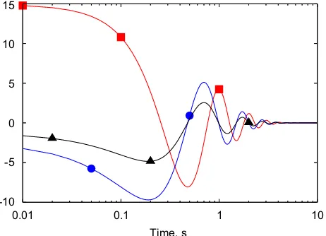
identification of the properties of the system. Fig. 1 illustrates the time history of the free response of the system for a perturbation of the initial value of the state; a 0.01 s time step is used. A logarithmic scale is used for the time axis to improve readability, since the highly damped response quickly vanishes.Fig. 2shows the coefficients of theRxx(left) andRxx_ (right) covariance matrices. They clearly undergo large variations, but
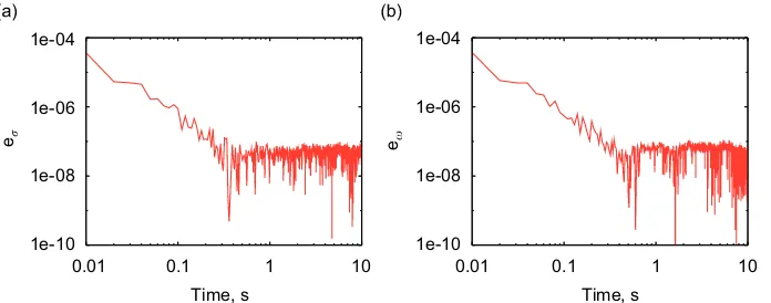
nonetheless the identification is very accurate right from the beginning, as shown inFig. 3, which presents the errors in the real (left) and imaginary (right) parts of the eigenvalue. They are very limited (below 1e4) for every time since the first time step, as soon as one measure, plus the initial conditions, is available to
-5
Fig. 1. Time history of the response of a damped, single degree of freedom, oscillating system: accelerationðmÞ; positionð’Þand velocity
numerically compute the covariance matrices, and do not significantly deteriorate even when the covariance coefficients tend to zero; they rather level down to the value reached when the time histories practically vanish.
3.3. Three masses problem
The problem, illustrated in Fig. 4, consists of three unit masses, constrained by three linear springs and dampers, whose stiffness and damping matrices are given by Eqs. (48) and (49)
K¼
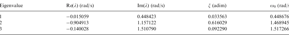
damping coefficients. The masses are only allowed to move along one direction, so the system has three degrees of freedom. The damping matrix has been designed to yield rather different damping values for the three modes that characterize the system, so that system identification becomes critical. The eigenvalues of the system are illustrated inTable 1.
-4
Fig. 2. Time history of theRxx(a) andR_xx(b) covariance matrix coefficients of a damped, single degree of freedom, oscillating system:
ð1;1Þ ð’Þ;ð1;2Þ ðÞ;ð2;2Þ ðmÞ.
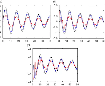
The system of differential equations is integrated in time with a time step of 0.01 s. As clearly shown by
Fig. 5, the effects related to the highly damped eigenvalues quickly disappear leaving just an oscillation on the frequency of the slow, lightly damped, first eigenvalue.
Table 2 shows the real and imaginary part of each eigenvalue identified by using the different techniques presented, while Table 3 gives the relative errors made by the identification techniques associated with each eigenvalue. Using the exact value of the acceleration of the masses at each time step, the estimates obtained with both techniques, Eqs. (20) and (21), are of high quality with an error on the real and imaginary parts of the eigenvalues which is below 1:5e10 (see first row of Table 3). The complex eigenvectors, illustrated in Fig. 6, also show a very low average relative error, below 1:0e8. Using a second order, centered finite difference approximation to compute the acceleration signal from the computed position and velocity, the error in the estimated eigenvectors increases, and a difference appears between the two different formulas (second and third line in Tables 2 and 3). Estimates obtained with Eq. (20) are always between two and three orders of magnitude more accurate than those obtained using Eq. (21). This is related to the fact that the covariance matrix Rx_x_ is more affected by the numerical
error introduced by the finite difference formula. The effect of this error is visible in the eigenvector estimate as well, at least for those obtained using Eq. (21).Fig. 6shows a comparison between the real and the computed eigenvectors in this last case. A significant error appears in the second eigenvector, which is highly damped.
In order to check the robustness of the method, a disturbance is added in terms of a random perturbing force (rpf) applied concurrently to the three bodies. This approach has been preferred to adding a measurement noise, because the velocity and position signal presented in the numerical examples are directly obtained by numerical simulation. In any case, results are expected to be similar to those obtained by considering measurement noise on acceleration signals from experiments. A limit case is presented with input force signal variancesFF¼0:1; lower force levels result in much better quality of the estimated eigensolutions.
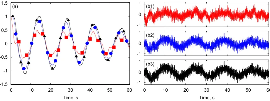
The resulting time histories of velocity and acceleration during the simulation are shown inFig. 7, which can be compared to the ‘‘clean’’ case inFig. 5. With this disturbance, the estimates obtained for the imaginary part of the eigenvalue by Eq. (20) are still acceptable, while the accuracy on the real part is generally poorer, especially on the less damped modes (seeTables 2 and 3). Note that the application of Eq. (21), which directly uses the acceleration signals, produces relative errors of more than 100%, yielding unreliable results. In this case, the filtering effect obtained by the numerical integration limits the impact of the disturbance on the estimated eigenvalues. Since the free response of the system vanishes, the quality of the covariance matrices and of the identification in this last case is largely affected by the duration of the time series, because the disturbance does not vanish and thus the signal to ‘‘noise’’ ratio quickly deteriorates the quality of the estimates.
Fig. 4. Three masses problem layout.
Table 1
Eigenvalues of the three masses problem;o0¼j jl,x¼ ReðlÞ=o0
Eigenvalue ReðlÞ(rad/s) ImðlÞ(rad/s) x(adim) o0(rad/s)
1 0:015059 0.448423 0.033563 0.448676
2 0:904913 1.157122 0.616029 1.468945
-3 -2 -1 0 1 2 3
0 10 20 30 40 50 60 0 10 20 30 40 50 60
0 10 20 30 40 50 60
-1 0 1 1.5
-0.8 0
0.5
-0.5
-1.5
0.8
0.4
-0.4
Fig. 5. Time response of the three masses system to an initial perturbation: position (a), velocity (b), and acceleration (c) of mass 1ð’Þ, 2ðÞ, 3ðmÞ.
Table 2
Eigenvalues evaluated by the different schemes
Case Eig. 1 Eig. 2 Eig. 3
ReðlÞ ImðlÞ ReðlÞ ImðlÞ ReðlÞ ImðlÞ
Exact acc. 0:01506 0.4484 0:90491 1.1571 0:14003 1.5108
Eq. (20) 2nd acc. 0:01506 0.4484 0:90491 1.1571 0:14002 1.5108
Eq. (21) 2nd acc. 0:01502 0.4475 0:90204 1.1535 0:13958 1.5060
Eq. (20)þ(rpf) 0:00916 0.4517 0:82790 1.1234 0:16375 1.5319
Eq. (21)þ(rpf) 0:00521 0.4735 0:99272 3.7192 0:00550 1.5484
Table 3
Relative error on the eigenvalues evaluated by the different schemes
Case Eig. 1 Eig. 2 Eig. 3
ReðlÞ ImðlÞ ReðlÞ ImðlÞ ReðlÞ ImðlÞ
Exact acc. 1:5e12 6:2e14 3:0e11 1:5e10 8:4e13 1:1e11
Eq. (20) 2nd acc. 3:2e06 8:4e07 7:5e06 1:4e05 2:4e05 9:3e06
Eq. (21) 2nd acc. 2:4e03 2:0e03 3:2e03 3:1e03 3:2e03 3:1e03
Eq. (20)þ(rpf) 3:9e01 7:2e03 8:5e02 2:9e02 1:7e01 1:4e02
Consider now the special case obtained giving the state
x¼ y
_
y
( )
(50)
an initial perturbation with a spatial resolution that exactly corresponds to the arbitrarily chosen ith eigenvector of this system
x0¼
y0
_
y0
( )
¼Ui. (51)
As a consequence, the whole system responds only at the frequency corresponding to the excited mode,
x¼Uielit, (52)
_
x¼liUielit, (53)
1 2 3
1 2 3 1
2
3
1 2
3
1
2 3
1 2
3
(1) (2) (3)
Fig. 6. Comparison between the reference eigenvectors (red, solid lines) and those computed using Eq. (21) using a second-order approximation of acceleration signals (blue, dashed lines).
-1.5 -1 -0.5 0 0.5 1 1.5
0 10 20 30 40 50 60
-1 0 1
-1 0 1
-1 0 1
0 10 20 30 40 50 60
Time, s Time, s
Fig. 7. Time response of the three masses system including random forcing: velocity (a) and acceleration (b 1,2,3) of mass 1ð’Þ, 2,
resulting in a spatial coherence of the measures, which makes the covariance matrices
Rxx¼UiUTi
1
t
Z t
0
e2litdt, (54)
Rxx_ ¼liUiUTi
1
t
Z t
0
e2litdt, (55)
Rx_x_ ¼l2iUiUTi
1
t
Z t
0
e2litdt (56)
singular, since UiUTi is singular by definition.
In this case, the use of a POD analysis allows to single out the significant signals included in the time histories. However, if the POD is applied to the covariance matrix built using only the position information, namelyRyy,
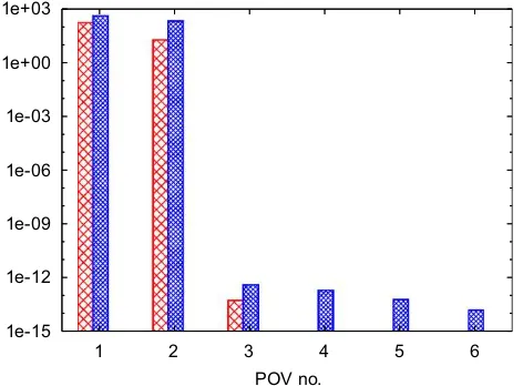
the resulting POVs are reported in Fig. 8 (bars on the left). The POD seems to indicate that there are two independent signals out of three; however, when Eq. (20) is applied to the time histories of the POMs related to the two non-zero POVs, the problem is still singular. Only applying the POD to the complete (i.e. positions and velocities) state covariance matrix,Rxx, the correct indication of two significant POMs out of six is obtained; the
corresponding POVs are also illustrated inFig. 8(bars on the right). The subsequent application of Eq. (20) to the time histories of the two active POMs extracted by the POD allows to correctly identify the eigenvalues corresponding to the modes activated by the perturbation. In conclusion, this approach does not directly deal with spatial resolution by itself, which is rather delegated to prior POD analysis.
4. Persistent excitation
In order to overcome the limitations of the free response analysis, similar techniques, based on covariance matrices, can be applied also when a persistent excitation is present. Consider a linear system with the addition of external inputs
_
x¼AxþBu. (57)
Eq. (8) is still valid; however, in order to give the correct interpretation of all terms, the effect of the system inputs must be taken into account. Recalling Eq. (5), the derivative ofxis now replaced by that in Eq. (57) to yield the error
ðlxAxBuÞTU¼e. (58)
1e-15 1e-12 1e-09 1e-06 1e-03 1e+00 1e+03
1 2 3 4 5 6
POV no.
The integral measure of the error becomes
J¼ lim
t!1
1 4t
Z t
t
e2dt. (59)
Applying exactly the same procedure as in Eq. (8), the expression
lim
t!1
1 2t
Z t
tð
lxAxBuÞðlxAxBuÞTdt
U¼0 (60)
results from the minimization ofJin Eq. (59). Integration over the sampling interval½t;tfort! 1yields
l2RxxlðARxxþBRuxþRxxATþRxuBTÞþARxxATþARxuBTþBRuxATþBRuuBT
U¼0. (61) Comparing Eqs. (8) and (61) one can observe that, by analogy
Rx_x_ ¼ARxxATþARxuBTþBRuxATþBRuuBT, (62)
Rxx_ þRxx_ ¼ARxxþRxxATþBRuxþRxuBT. (63)
4.1. White noise
To obtain a persistent excitation, consider as input signal a white noise, namely a signal whose covariance matrix is
Kuu ¼ lim
t!1
1
t
Z t
t
uðvÞuTðvþtÞdv (64)
¼WdðtÞ, (65)
whereWis the noise intensity matrix, anddðtÞis Dirac’s delta distribution:
Z 1
1
dðtÞdt¼1, (66)
Z 1
1
fðtÞdðtÞdt¼fð0Þ. (67)
In this special case, the covariance matrix computed with no time shift, i.e. for t¼0, is not defined as a function; however, with a small abuse of mathematical notation, it is possible to define
Ruu¼ def
lim
t!0WdðtÞ ¼WdL, (68)
where dL¼dð0Þ in theory means þ1, but never needs to be practically evaluated, as illustrated in the following.
In this case the cross-covariance between the state vector and the input signal becomes exactly equal to
Rxu¼12BW. (69)
Eq. (61), which is valid only in the limit sense, then becomes
l2RxxlðARxxþRxxATþBWBTÞ þARxxATþ12ABWBTþ12BWBTATþBWBTdL¼0 (70)
while Eqs. (62) and (63) become
Rx_x_ ¼ARxxATþ12ABWBTþ12BWBTATþBWBTdL, (71)
Rxx_ þRxx_ ¼ARxxþRxxATþBWBT. (72)
In this case alsoRx_x_ cannot be defined as a function, so it is necessary to see it as
Rx_x_def¼lim
and
Kx_x_ðtÞ ¼ lim t!1
1 2t
Z t
t
_
xðvÞx_TðvþtÞdv. (74)
When the signals are stationary, as they are in this case since the system is excited by a stationary white noise, exploiting Eq. (24) in Eq. (72) gives the well known Lyapunov’s algebraic equation for the computation of state covariances3[19]
ARxxþRxxATþBWBT¼0. (75)
Remembering that Rxx_ ¼RTxx_ , Eq. (72) allows to infer
Rxx_ ¼RxxATþ12BWBT. (76)
The matrix equations obtained so far can be used to identify the state matrix of the observed system.
4.2. Measured excitation
When the time history of the input signaluis known, which means that the covarianceWof the excitation is known as well, one can use the definition of the input-output covariance Rxu to estimate matrixB
Rxu¼12BW)B¼2RxuW1, (77)
and then matrixAfrom a simple elaboration of the transpose of Eq. (76)
A¼ ðRxx_ 2RxuW1RuxÞRxx1. (78)
4.3. Unknown excitation
In many cases of practical interest, it may be reasonably assumed that the applied disturbance is a white noise without any additional information on the time history of the input signals. Consider Eq. (76) and use it to replace BWBTin Eq. (75)
ARxxRxxATþRxx_ Rxx_ ¼0, (79)
whereRxx_ ¼RTxx_ andRTxx_ ¼ Rxx_ have been exploited. This equation is skew-symmetric, and can be used to
infer information about the state matrixAgiven the covariances. It actually containsnðn1Þ=2 equations in then2 unknowns represented by the coefficients of matrixA, so it is not sufficient by itself to determine the
unknown matrix. Consider now
Rxx_ ¼RTxx_ ¼ARxxþ12BWBT (80)
and use it along with Eq. (76) to eliminate the first two occurrences ofBWBTfrom Eq. (71); use Eq. (72) along with Eq. (68) to eliminateBWBTdL as well. Eq. (71) becomes:
ARxxATAðRxx_dLRxxÞ ðRxx_ dLRxxÞATþRx_x_ ¼0. (81)
Eq. (81) represents a second-order algebraic equation in matrix A which is based on the covariance and cross-covariance matrices of the measurements x and their derivatives. It is symmetric, so it actually contains the remaining nðnþ1Þ=2 equations that are necessary to determine all the coefficients of matrixA.
An asymptotic analysis of Eq. (81) shows that it is dominated by the terms multiplied bydL; this term is also
implicitly contained inRx_x_, so when the analytical covariances are considered, for a true, i.e. infinite band,
white noise, it degenerates into
ARxxþRxxATþlim
t!0
1
dðtÞKx_x_ðtÞ ¼0, (82)
where the limit exists and is finite. Eq. (82) is again the well-known Lyapunov’s algebraic equation.
The union of the skew-symmetric Eq. (79) and of the symmetric Eq. (81), or of the corresponding asymptotic one (82), yields a system of equations that is consistent. If Eq. (82) can be considered, the system is linear; otherwise, a weakly quadratic problem results, where the importance of the quadratic term grows as the noise bandwidth decreases.
In conclusion, considering an unknown linear system subjected to white random noise in input, using the information contained in the covariance matrices, through Eqs. (79), (81), the state matrix can be identified. This very interesting result, to the authors’ knowledge, has never been shown before.
4.4. Band limited white noise
A term that goes to infinity,dL, appears in Eq. (81). This is due to the fact that the covariance of an ideal white noise goes to infinity, so a process like that is not physically realizable. However, it can be approximated by what is usually called a wide band white noise with exponential correlation [15], defined by a covariance matrix
KuuðtÞ ¼W
a
2e
ajtj, (83)
wherea is the band limit[15]. This process becomes a white noise when a! 1. The variance between the system state and the input signal is
Rxu¼ lim
If the band limit is large enough compared to the characteristic frequencies of the system under analysis, the term under the integral expression can be approximated by eajvj, so the covariance becomes
Rxu 12BW, (84)
which corresponds to the expression obtained for the white noise, Eq. (69). The covariance matrix of the band limited noise fort¼0 becomes equal to
Ruu ¼W
a
2¼WdF, (85)
where the value ofdF is now limited by the bandwidthaof the noise.
In all the numerical examples presented in the following section the white noise has been simulated using a set of normally distributed random numbers generated at each time step by the Matlab function randn. A simple relation between the discrete and the continuous domain shows that the noise bandwidth is 2=Dt, and
thusdF ¼1=Dt. These values have been confirmed by simple numerical experiments, where the power spectral
density of the generated noise has been computed and evaluated.
4.5. Numerical solution for the unknown excitation case
In the most general case, when a wide band white noise is considered as input, and the noise input is unknown, the system of matrix equations
LðARxxRxxATþRxx_ Rxx_ Þ ¼Lð0Þ. (86)
must be solved, where operatorsUðÞandLðÞ, respectively, return the upper and the strictly lower triangular parts of the argument. The problem is in general nonlinear; the solution can be obtained using a Newton-like iterative numerical method. For conciseness, the problem of Eq. (86) is rewritten as
UðASATARRTATþQÞ ¼Uð0Þ
LðASSATþPÞ ¼Lð0Þ, (87)
where
S¼Rxx, (88)
R¼Rxx_ dFRxx, (89)
Q¼Rx_x_, (90)
P¼Rxx_ Rxx_ . (91)
After indicating with
uij¼aikskhajhaikrkjrkiajkþqij¼0 (92)
lij¼aikskjsikajkþpij, (93)
the generic equations from the symmetric (uij,jXi) and the skew-symmetric (lij,joi) problems, respectively,
the Jacobian matrix can be analytically computed as
quij
qamn¼dimsnhajhþdjmaikskndimrnjdjmrni, (94) qlij
qamn¼dimsnjdjmsin, (95)
wheredijis Kronecker’s operator, and implicit summation is assumed over repeated subscripts.
The problem of selecting the ‘‘right’’ solution of the nonlinear problem is yet to be solved; however, in the numerical cases addressed so far this point does not appear to be critical. The same applies to the initial guess of matrixA. The skew-symmetric equation (79) is not required if a second-order model is enforced. In fact, the typical state-space representation of second-order structural problems, where
x¼ y
z
(96)
yields exactlynðnþ1Þ=2 unknowns, because matrixAcan be partitioned as
A¼ 0 D
A21 A22
" #
, (97)
whereDis a diagonal matrix that contains the scale factors between the derivatives of the positions,y_, and the pseudo-velocitiesz, typically equal to the identity matrixIwhenz¼y_.
It appears that any linear combination of Eqs. (79) and (81) represents a general, non-symmetric algebraic Riccati-like4equation. The analytical solution of simple cases presented in the following seems to indicate the presence of a reflection axis for the eigenvalues of the two solutions of matrixA, crossing the real axis atdF
and parallel to the imaginary axis. This suggests that some shift technique, capable of bringing the reflection plane onto the imaginary axis, could turn the problem into Hamiltonian form, and thus naturally allow to select the stable solution by using standard techniques for algebraic Riccati equations. However, this direction needs further investigation.
The analytical application of the above techniques to a first- and second-order scalar problem, and their numerical application to the three masses problem, is illustrated to clarify their properties.
4.6. Scalar, first-order problem
Consider the scalar problem
_
y¼lyþbu. (98)
The covariance matrix can be computed from Lyapunov’s equation (75)
lsyyþsyylþb2w¼0, (99) whereais the unknown coefficient. It results from the solution of the second-order polynomial equation
a2þ2dFalðlþ2dFÞ ¼0, (103)
The first one is the ‘‘right’’ root, while the other, which tends to 1 according to the ratio between the noise bandwidth and the system eigenvalue, is essentially meaningless. In fact, when using the asymptotic equation (82)
the correct system root is obtained directly.
4.6.2. Measured excitation
Ifu is measured, and thuswis known, Eq. (77) yields
while Eq. (78) yields
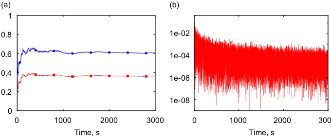
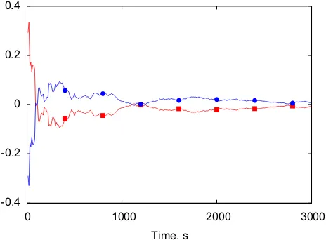
A first numerical application has been made on this very simple system. In this casel¼ 2 andb¼1:2. The system is integrated numerically with a time step of 0.01 s.Fig. 9(a) shows how the state covariance and the cross-covariance between the state and the input converge toward an almost constant value. At least a time of 1000 s is necessary to obtain a significant stabilization in the covariances. However, the analysis ofFig. 9(b) gives an indication about the non-perfect ‘‘whiteness’’ of the input noise. In fact, the cross-covariance between the derivative of the state and the state itself must go to zero. The figure shows that the trend is correct; however, after the initial times, the values seem to reach a plateau. At the same time the measured power spectrum of the noise between 0 and the band limit is far from being regular (either similar to a quadratic decay, as the one associated with the exponential correlation or to a uniform value as the one associated with a band limited white noise [15]). The resulting relative errors in the identified values of l and b are shown inFig. 10. The error drops below 5% after 1000 s (and 100,000 steps), and goes around 1% after 3000 s, with a very slow decay. Such a large time window is taken just to show that the decay of the error after the first time portion is very slow. Interestingly enough, the two relative errors are exactly opposite.
4.7. Scalar, second-order problem
Consider the scalar second-order problem
my€þcy_þky¼f (108)
From Lyapunov’s equation and from the definitions of the covariances
sy_y_ ¼
From Eq. (81), by imposing that matrixAtakes the form
wherea11 ¼0 is assumed because matrixAis the first-order representation of a second-order scalar equation,5
The result of Eq. (120) is expected; however it may not be trivial if, for example, some scaling occurs between the derivatives of the measurements. Eq. (121) yields the exact result for the stiffness-mass ratio; this is also expected. Eq. (122) allows two results; one is the exact value of the damping-mass ratio, while the other is essentially irrelevant. Again it tends to1, so it is easily distinguishable from the correct one.
4.7.2. Measured excitation
Iffis measured, the exact values are obtained for matricesBandA:
B¼2 syf
Consider now the three masses problem ofFig. 4, already used as a test example in earlier sections. In this cases no analytical solution is sought; only numerical solutions are considered.
4.8.1. Unknown excitation
In this case, the computation of the covariance matrices suffers from the quality of the noise that is used to force the system. The method assumes that the unknown excitation is white noise, so the results of the identification may significantly depart from the exact value if the power spectral density of the noise is not uniform.
5This is required because Eq. (81) is symmetric, and thus it actually representsn
The problem has been solved by numerically computing the solution of Eqs. (81) and (79) directly, by means of Matlab’sfsolvecommand. The problem consists in 36 equations with 36 unknowns, and the initial guess consisted in a matrix with the structure
A0¼
0 I
0 0
. (127)
The result appears to be quite robust with respect to the initial guess of the solution: in no case the procedure converged to a different solution. Of course, this does not represent a proof, neither of uniqueness nor of stability of the solution; further investigation is required to assess the properties of the equation and of its numerical solution.
Three, almost uncorrelated, band-limited white noise forces with different intensity have been applied to the three masses. The intensity matrixWis reported in the following equation:
W¼
even thought it has not been used for the identification in the cases presented in the following.
The matrix A resulting from the numerical solution of the problem obtained by joining the two Eqs. (81), (79) is
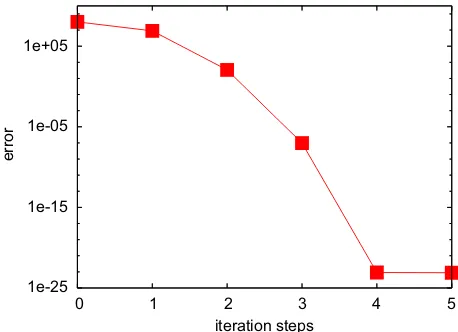
which shows the structure of Eq. (97), with a null 33 matrix in the upper left corner and the identity matrix in the upper right corner. The most significant coefficients of the stiffness and damping matrices are visible too. The convergence in the solution of the nonlinear problem of Eq. (86) is extremely fast, as shown inFig. 11
where the trend of the norm of the problem residual is shown. InTable 4, the results of the eigensolutions resulting from the matrix identified using covariance matrices after 500 and 3000 s of elapsed time are compared with the exact ones.Table 5 shows analogous results obtained with a classical discrete subspace identification method, N4SID[20], considering a stochastic unknown input. The comparison of the two tables shows that the quality of the results is comparable, with a slight advantage on the method here proposed. The error is generally low for the imaginary part and can be considered acceptable for the real part related to the damping. The error on the computed eigenvectors is shown inFig. 12.
4.8.2. Measured excitation
The resulting matrixBis
B¼
1:4584e1 5:9196e2 1:3117e1
9:2979e2 5:8983e2 2:2654e1
1:3850e1 8:5302e2 2:1200e1 1:1379eþ0 7:3443e2 4:4223e3 3:6637e2 9:8293e1 1:1803e1 7:0270e2 1:0066e3 1:1032eþ0
2
6 6 6 6 6 6 6 6 4
3
7 7 7 7 7 7 7 7 5
,
1e-25 1e-15 1e-05 1e+05
0 1 2 3 4 5
error
iteration steps
Fig. 11. Residual norm during the solution of the nonlinear problem of Eq. (86).
Table 5
Identified eigenvalues of the three masses problem with stochastic N4SID
Elapsed time (s) Eig. ReðlÞ(rad/s) ImðlÞ(rad/s) err. ReðlÞ err. ImðlÞ
500 1 0:01164 0.4464 0.2268 8:428e3
2 0:92309 1.3342 0.0200 1:530e1
3 0:08687 1.4988 0.3796 7:96213
3000 1 0:01399 0.4495 0.0706 2:419e3
2 0:93806 1.2065 0.0366 4:263e3
3 0:10022 1.5341 0.2842 2:512e3
Table 4
Identified eigenvalues of the three masses problem with the unknown input noise
Elapsed time (s) Eig. ReðlÞ(rad/s) ImðlÞ(rad/s) err. ReðlÞ err. ImðlÞ
500 1 0:01237 0.4446 0.17860 8:577e3
2 0:87735 1.2473 0.03046 7:797e2
3 0:11655 1.5295 0.16767 1:238e2
3000 1 0:01377 0.4494 0.08537 2:126e3
2 0:91287 1.1590 0.00880 1:635e3
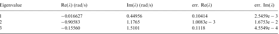
Table 6
Identified eigenvalues of the three masses problem with measured excitation after 3000 s
Eigenvalue ReðlÞ(rad/s) ImðlÞ(rad/s) err. ReðlÞ err. ImðlÞ
1 0:016627 0.44956 0.10414 2:5459e3
2 0:90583 1.1765 1:0083e3 1:6753e2
3 0:15560 1.5101 0.1118 4:5549e4
1 2
(1) (2) (3)
3
1 2 3 1
2
3
1 2
3 1
2 3
1
2 3
Fig. 12. Comparison between the reference eigenvectors (red, solid lines) and those computed with the unknown noise excitation method (blue, dashed lines).
1e-06 1e-04 1e-02 1e+00 1e+02
0 1000 2000 3000
1e-06 1e-04 1e-02 1e+00 1e+02
0 1000 2000 3000
1e-06 1e-04 1e-02 1e+00 1e+02
0 1000 2000
Time, s Time, s
Time, s
3000
(1) (2)
(3)
which closely resembles the expected one,
B¼ 0
M1
.
The comparison of the computed eigenvectors is presented inFig. 14where again the higher error is the vector which presents the lowest error in the real and imaginary part, which is also the most damped one.
The measured excitation method seems to perform slightly worse than the one which does not directly use the information related to the input. This is probably due to the fact that the computed matrixRxucontains larger errors than the one that can be theoretically obtained from Eq. (69). In this case the
N4SID algorithm using the information gained from the input time history outperforms the method here presented.
5. Final remarks
The work here presented stems from the need to interpret proper orthogonal modes to understand how it is possible to recover information related to the eigensolution of the system under analysis. As a result, an approach to the identification of the eigensolutions of systems from free and forced response is presented, based on deterministic auto- and cross-covariances. The use of cross-covariances allows accurate estimates of state space representations of linear systems when they are not stationary. This allows to add the required information to the characteristic covariance matrices needed to recover the correct eigensolutions from the proper orthogonal decomposition in any condition. Identification from free responses may suffer from the presence of disturbances; this is mitigated by considering the forcing terms in the identification. When the knowledge of the input is not exploited interesting results are obtained from the simultaneous solution of a Lyapunov-like and a non-symmetric Riccati-like algebraic equation (when the input represents a good approximation of band-limited white random noise). To our knowledge the problem has not been presented in this form yet. Analytical and numerical results illustrate the soundness of the approach in simple, yet significant applications.
The ‘‘unknown excitation’’ method seems to perform always better than the one tagged as ‘‘measured excitation’’, so it should be used in any case. However, the last one gives the additional estimate of the input distribution matrix. Improvement on this side may come from better numerical representation of white noise processes or from exploiting Eqs. (62), (63), for a general non-white noise measured input. Issues related to the capability of the input to excite all the included system dynamics certainly will arise anyhow.
Some open issues remains on the correct mathematical characterization and on a possible general solution for the ‘‘unknown excitation’’ identification equation. Future investigations will include the possibility to use the defined proper dynamic decomposition, as a system reduction method for dynamic systems, looking in
1 2 3
1 2 3 1
2
3
1 2
3 1
2 3
1
2 3
(1) (2) (3)
more details to its properties, and the possible insight into the system under investigation when nonlinear cases are considered.
References
[1] G. Kerschen, J.-C. Golinval, A. Vakakis, L. Bergman, The method of proper orthogonal decomposition for dynamical characterization and order reduction of mechanical systems: An overview,Nonlinear Dynamics41 (1–3) (2005) 147–169.
[2] I.T. Jolliffe,Principal Component Analysis, second ed., Springer, New York, NY, 2002.
[3] K. Pearson, On lines and planes of closest fit to system of points in space,Philosophical Magazine2 (6) (1901) 559–572.
[4] H. Hotelling, Analysis of a complex of statistical variables into principal components, Journal of Educational Psychology 24 (1933) 417–441, 498–520.
[5] S. Bellizzi, R. Sampaio, POMs analysis of randomly vibrating systems obtained from Karhunen-Loe`ve expansion,Journal of Sound and Vibration297 (2006) 774–793.
[6] Y.K. Lin,Probabilistic Theory Of Structural Dynamics, McGraw-Hill, New York, NY, 1967.
[7] B. Feeny, R. Kappagantu, On the physical interpretation of proper orthogonal modes in vibrations,Journal of Sound and Vibration
211 (4) (1998) 607–616.
[8] G. Kerschen, J. Golinval, Physical interpretation of the proper orthogonal modes using the singular value decomposition,Journal of Sound and Vibration249 (5) (2002) 849–865.
[9] B. Feeny, Y. Liang, Interpreting proper orthogonal modes of randomly excited vibration systems,Journal of Sound and Vibration265 (2003) 953–966.
[10] G. Quaranta, P. Masarati, P. Mantegazza, Dynamic characterization and stability of a large size multibody tiltrotor model by POD analysis,ASME 19th Biennial Conference on Mechanical Vibration and Noise(VIB), Chicago IL, 2003.
[11] G. Quaranta, P. Masarati, P. Mantegazza, Assessing the local stability of periodic motions for large multibody nonlinear systems using POD,Journal of Sound and Vibration271 (3–5) (2004) 1015–1038.
[12] S. Han, B. Feeny, Application of proper orthogonal decomposition to structural vibration analysis,Mechanical System and Signal Processing17 (5) (2003) 989–1001.
[13] D. Chelidze, W. Zhou, Smooth orthogonal decomposition-based vibration mode identification,Journal of Sound and Vibration292 (3–5) (2006) 461–473.
[14] F. Tisseur, K. Meerbergen, The quadratic eigenvalue problem,SIAM Review43 (2) (2001) 235–286.
[15] A. Preumont,Random Vibration and Spectral Analysis of Solid Mechanics and its Applications, Vol. 33, Kluwer Academic Publishers, Dordrecht, The Netherlands, 1994.
[16] R. Skelton, I. Iwasaki, K. Grigoriadis,A Unified Algebraic Approach to Linear Control Design, Taylor & Francis, London, UK, 1998. [17] L. Ljung,System Identification: Theory for the User, Prentice-Hall, Inc., Upper Saddle River, NJ, USA, 1986.
[18] G.H. Golub, C.F. van Loan,Matrix computation, second ed., John Hopkins University Press, Baltimore, 1991. [19] A. Bryson, Y. Ho,Applied Optimal Control, Wiley, New York, 1975.
[20] P. Van Overschee, B. De Moor, N4SID: subspace algorithms for the identification of combined deterministic-stochastic systems,