APPLICATION OF FORWARD – BACKWARD PROPAGATION ALGORITHM FOR THREE – PHASE POWER FLOW ANALYSIS IN RADIAL DISTRIBUTION SYSTEM

APPLICATION OF FORWARD – BACKWARD PROPAGATION

ALGORITHM FOR THREE – PHASE POWER FLOW ANALYSIS IN

RADIAL DISTRIBUTION SYSTEM

Agus Ulinuha

Department of Electrical Engineering, Muhammadiyah University of Surakarta

Jl. A. Yani Pabelan, PO BOX 1 Kartasura Surakarta, Postcode 57102 Phone: +62 271 717417 Fax +62 271 715448 Email: ulinagus1970@gmail.com

Abstrak

Power flow analysis is backbone of power system analysis and design. It is essential for power system analysis in operational as well as in planning stages. Power flow calculation is normally performed by simply considering that the system under study is completely balance. Actual distribution system is inherently unbalance and therefore three-phase power flow is necessary to accurately simulate the unbalance system. However, inclusion of unbalance increases the dimension of problem and, as distribution system is commonly constructed as radial system with high R/X ratio, it may also cause the sophisticated power flow algorithms fail to converge. The robust algorithm for three-phase power flow is therefore needed. In this paper, three-phase power flow for unbalance distribution system is carried out using Forward-Backward Propagation Technique. The equivalent injection current method is employed to represent the loads and shunt admittances. The algorithm starts with mapping the distribution network to determine the forward and backward propagation paths. The backward propagation is used to calculate branch currents using the bus injection currents. The forward propagation is employed to calculate bus voltages using the obtained branch currents and line impedances. The algorithm offers robust and good convergence characteristics for radial distribution system. The algorithm is presented for the IEEE 34-bus system with satisfied generated results. Keyword: Convergence; equivalent injection current; forward-backward propagation; unbalance

system Introduction

Power flow calculation is backbone of power system analysis and design. It is essential for analysis of any power system in the operational as well as planning stages. The calculation is initially carried out by formulating the network equation. Node-voltage method, which is the most suitable form for many power system analyses, is commonly used. Mathematically, power flow problem requires solution of simultaneous nonlinear equations and normally employs an iterative method, such as Gauss-Seidel and Newton-Raphson.

Power flow calculation is normally performed by simply considering that the system under study is balance. Hence, the calculations are carried out for single phase assuming that the other two phases are exactly the same but with the 120 degrees phase difference. The asymmetry in lines and loads produces a certain level of unbalance in real power system and this is considered as disturbance whose level should be controlled to maintain the electromagnetic compatibility of the system (Mayordomo, Izzeddine et al. 2002).

For distribution system, in particular, the system is inherently unbalanced, due to factors such as the unbalance of customer loads, the presence of unsymmetrical line spacing, and the combination of single, double and three-phase line sections. Therefore, three-phase power flow is necessary to accurately simulate the unbalance system.

Inclusion of unbalance increases the dimension of problem as all the three phases need to be considered instead of single phase balanced representation. On the other hand, distribution system commonly constructed as radial system with high R/X ratio may cause the sophisticated power flow algorithms fail to converge. The robust algorithm for three-phase power flow is therefore needed.

symmetrical components. All components are modeled by phase voltages, admittances and independent current sources. This approach will work well as long as every component can be modeled in the admittance matrix or can be converted into equivalent injection current.

The methods for three-phase distribution networks can be basically divided into two classes, Gauss-Seidel (Teng 2002; Vieira, Freitas et al. 2004) and Newton-Raphson (Garcia, Pereira et al. 2000; Lin and Teng 2000; da Costa, de Oliveira et al. 2007). Gauss-Seidel method needs much iteration and is known to be slow. Newton-Raphson has good convergence characteristic, but the Jacobian that needs to be partially or totally calculated in every iteration makes this approach unattractive.

This paper presents three-phase power flow for unbalance distribution system using forward-backward propagation technique. The algorithm works directly on the system without any modification. Therefore, there is no need to decompose the system into symmetrical components as well as to decouple the system into individual phases. However, the conversion of load and shunt element into their equivalent injection current is necessary. Distribution line charging is usually too small to be included (Lin and Teng 2000). The algorithm is implemented on IEEE 34-bus system including asymmetrical lines and unbalance loads.

System Modeling Line Modeling

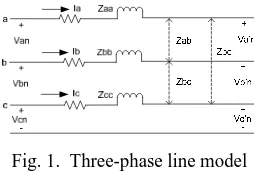
The accuracy of three-phase power flow results greatly depends on the line impedance model used. Therefore, an exact model of a three-phase line section needs to be firstly developed. The model of distribution line feeder as in (Kersting and Phillips 1995) will be developed and used in this paper. An equivalent circuit for a three-phase line section is shown in Fig. 1.

Fig. 1. Three-phase line model

The modeling of three-phase lines starts with determination of self and mutual impedances of a line section which are functions of the conductors and the spacing between conductors on the pole or underground. The “modified” form of Carson’s equations are used to determine the self and mutual impedances of this model and are given by the following equations:

[

ln(1/ ) 7.934

]

Where ri is the conductor resistance (Ω/mile), GMRi is the conductor geometric mean radius (ft), and Dij is the spacing between conductors i and j (ft). Application of (1) and (2) to the three-phase line indicated in Fig. 1. results in a 4×4 “primitive impedance matrix”:

[

]

By applying Kron reduction, this matrix may be reduced into 3×3 “phase impedance matrix” whose elements are determined by the following equation:

nn

And the resulted “phase impedance matrix” is:

Load Modeling

The load (balance and unbalance) is represented by its equivalent injection current. The load modeling as in (Vieira, Freitas et al. 2004) is adopted in this paper. For three-phase loads connected in wye or single-phase loads connected line to neutral, the equivalent injection currents at kth bus are determined by the following equation:

*

Where Pm, Qm, Vm* denote real power, reactive power, and complex conjugate of the voltage phasor for each phase, respectively. For three-phase loads connected in delta or single-phase loads connected line to line, the equivalent injection currents at the kth bus are determined by the following equations:

*

Where Pn, Qn, n ∈ [ab, bc, ca], represents the real and reactive load connected between the respective phases, and Vm* , m ∈ [a, b, c] denotes the complex conjugate of the voltage phasor for each phase, respectively.

Shunt Admittance Modeling

Three phase shunt capacitors can also be represented by equivalent injection currents (Vieira, Freitas et al. 2004). Assuming that the capacitor bank has an ungrounded wye connection, the current injection in each phase can be expressed by:

(

k

)

each phase. If the capacitor bank has a grounded wye connection, then the injection current is:

k

Power flow is calculated by initially mapping the distribution network to determine forward and backward propagation paths followed by branch current calculation and bus voltages calculation.

Branch Current Calculation

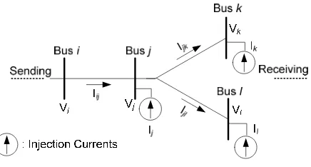
Fig. 2. Part of a distribution system

Fig. 2 indicates a part of distribution system and bus injection currents. The relationships between branch currents and injection currents are:

k jk I I =−

l jl I

I =− (10)

k jl jk

ij I I I

I = + −

Where Ijk is the branch current between bus j and bus k, and Ij injection currents at bus, respectively.

Bus Voltage Calculation

Using forward propagation path, the voltage at each bus is calculated using the obtained branch currents and line impedance. The voltages are consecutively calculated from the source (swing) toward the network ends. The voltage of swing bus is kept constant at 1.0∠00 pu, 1.0∠-1200 pu, and 1.0∠1200 pu for phase a, b, and c, respectively. For the part of system indicated in Fig. 2, the bus voltages can be calculated as follows:

ij ij i j V Z I

V = −

jk jk j

k V Z I

V = − (11)

jl jl j

l

V

Z

I

V

=

−

Where Vj is the voltage at bus j and Zjk is the impedance of line section between bus j and k. The updated bus voltages are then used to calculate the bus injection currents. It should be noted that all calculations are carried in the three-phase frame.

Convergence Criteria

The outlined steps for branch currents and bus voltages calculations are invoked during the power flow iteration. The iteration converges if the different of bus voltages for the consecutive iterations is equal to or less than the prescribed tolerance. The voltage mismatch of bus j at the nth iteration is given by:

1

−

− =

Δ n

j n j n

j V V

V for phase a, b, c ε

<

Δ )

(

Re Vn_j ; j ∈ all buses (12)

ε

<

Δ )

(

Im V_jn ; j ∈ all buses

Fig. 3. The flowchart for three-phase power flow calculation using Forward-Backward Propagation technique

Simulation System Data

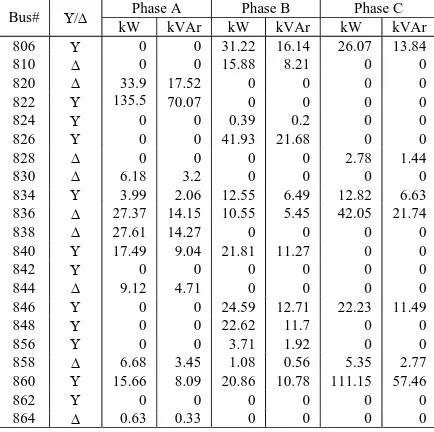
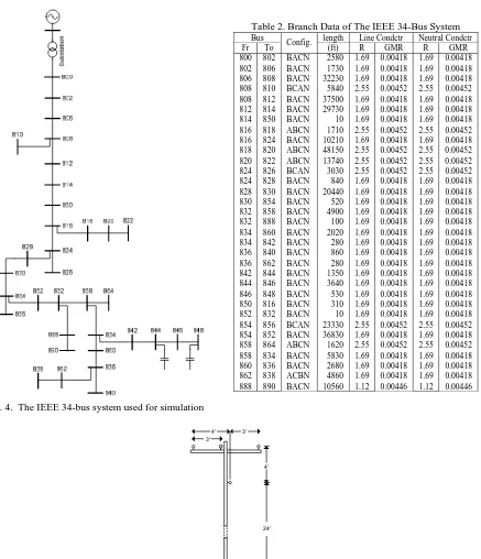
The simulation is carried out for the IEEE 34-bus system (Kersting 1991) indicated in Fig. 4. The system includes balance as well as unbalance loads. A minor modification is performed for the system to only include three phase asymmetrical lines. However, the load data and the capacitor data are remain the same. The system load and branch data are respectively given in Table 1 (A and B) and Table 2.

Table 1(a) Balance Loads of the IEEE 34-bus System Phase A Phase B Phase C Bus# Υ/Δ

kW kVAr kW kVAr kW kVAr 860 Υ 19.91 15.94 19.91 15.94 19.91 15.94

840 Υ 8.86 7.09 8.86 7.09 8.86 7.09

844 Δ 133.444 106.83 133.444 106.88 133.444 106.88 848 Υ 19.45 15.57 19.45 15.57 19.45 15.57

890 Δ 27 21.62 27 21.62 27 21.62

Note

1. Swing: bus 800 2. MVA base: 2.5 MVA

Table 1(b) Unbalance Loads of the IEEE 34-bus System Phase A Phase B Phase C Bus# Υ/Δ

kW kVAr kW kVAr kW kVAr 806 Υ 0 0 31.22 16.14 26.07 13.84

810 Δ 0 0 15.88 8.21 0 0

820 Δ 33.9 17.52 0 0 0 0

822 Υ 135.5 70.07 0 0 0 0

824 Υ 0 0 0.39 0.2 0 0

826 Υ 0 0 41.93 21.68 0 0

828 Δ 0 0 0 0 2.78 1.44

830 Δ 6.18 3.2 0 0 0 0

834 Υ 3.99 2.06 12.55 6.49 12.82 6.63 836 Δ 27.37 14.15 10.55 5.45 42.05 21.74

838 Δ 27.61 14.27 0 0 0 0

840 Υ 17.49 9.04 21.81 11.27 0 0

842 Υ 0 0 0 0 0 0

844 Δ 9.12 4.71 0 0 0 0

846 Υ 0 0 24.59 12.71 22.23 11.49

848 Υ 0 0 22.62 11.7 0 0

Fig. 4. The IEEE 34-bus system used for simulation

Table 2. Branch Data of The IEEE 34-Bus System Bus length Line Condctr Neutral Condctr Fr To Config. (ft) R GMR R GMR 800 802 BACN 2580 1.69 0.00418 1.69 0.00418 802 806 BACN 1730 1.69 0.00418 1.69 0.00418 806 808 BACN 32230 1.69 0.00418 1.69 0.00418 808 810 BCAN 5840 2.55 0.00452 2.55 0.00452 808 812 BACN 37500 1.69 0.00418 1.69 0.00418 812 814 BACN 29730 1.69 0.00418 1.69 0.00418 814 850 BACN 10 1.69 0.00418 1.69 0.00418 816 818 ABCN 1710 2.55 0.00452 2.55 0.00452 816 824 BACN 10210 1.69 0.00418 1.69 0.00418 818 820 ABCN 48150 2.55 0.00452 2.55 0.00452 820 822 ABCN 13740 2.55 0.00452 2.55 0.00452 824 826 BCAN 3030 2.55 0.00452 2.55 0.00452 824 828 BACN 840 1.69 0.00418 1.69 0.00418 828 830 BACN 20440 1.69 0.00418 1.69 0.00418 830 854 BACN 520 1.69 0.00418 1.69 0.00418 832 858 BACN 4900 1.69 0.00418 1.69 0.00418 832 888 BACN 100 1.69 0.00418 1.69 0.00418 834 860 BACN 2020 1.69 0.00418 1.69 0.00418 834 842 BACN 280 1.69 0.00418 1.69 0.00418 836 840 BACN 860 1.69 0.00418 1.69 0.00418 836 862 BACN 280 1.69 0.00418 1.69 0.00418 842 844 BACN 1350 1.69 0.00418 1.69 0.00418 844 846 BACN 3640 1.69 0.00418 1.69 0.00418 846 848 BACN 530 1.69 0.00418 1.69 0.00418 850 816 BACN 310 1.69 0.00418 1.69 0.00418 852 832 BACN 10 1.69 0.00418 1.69 0.00418 854 856 BCAN 23330 2.55 0.00452 2.55 0.00452 854 852 BACN 36830 1.69 0.00418 1.69 0.00418 858 864 ABCN 1620 2.55 0.00452 2.55 0.00452 858 834 BACN 5830 1.69 0.00418 1.69 0.00418 860 836 BACN 2680 1.69 0.00418 1.69 0.00418 862 838 ACBN 4860 1.69 0.00418 1.69 0.00418 888 890 BACN 10560 1.12 0.00446 1.12 0.00446

3'

4' 3'

4'

24'

Fig. 5. Overhead line spacing for the IEEE 34-bus system

Fig. 5 shows the spacing distances between the phase conductors and the neutral conductor. The line configuration is given in Table 2 (3rd _{column) indicating that the phase conductors are sequentially placed starting}

Simulation Results

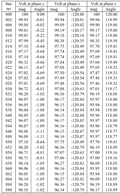
The system is run using the algorithm presented in Fig. 3. The simulation is coded using Matlab version 7.0 (R14). For the system of Fig.4, the three-phase power flow calculation takes 5 iterations to converge. This iteration number is fairly small indicating that the algorithm is robust for unbalance power flow calculation. The results of simulation including magnitude and angle of voltage at every phase are given in Table 3. The simulation also indicates the real and reactive power losses of 8.2 kW and 3.4 kVAr, respectively.

Table 3. Simulation Results of The IEEE 34-Bus Unbalance System Volt at phase c Volt at phase c Volt at phase c bus

no mag Angle mag Angle mag Angle 800 100 0.00 100 -120.00 100 120.00 802 99.93 -0.01 99.94 -120.01 99.94 119.99 806 99.88 -0.02 99.89 -120.02 99.90 119.98 808 99.01 -0.22 99.19 -120.17 99.17 119.80 810 99.01 -0.22 99.18 -120.18 99.17 119.80 812 97.99 -0.45 98.38 -120.35 98.35 119.58 814 97.18 -0.64 97.75 -120.49 97.70 119.41 816 97.17 -0.64 97.74 -120.49 97.69 119.41 818 97.14 -0.64 97.74 -120.49 97.69 119.41 820 96.32 -0.66 97.84 -120.49 97.66 119.49 822 96.11 -0.67 97.88 -120.49 97.65 119.52 824 97.02 -0.69 97.50 -120.54 97.47 119.33 826 97.02 -0.69 97.49 -120.54 97.48 119.33 828 97.01 -0.69 97.48 -120.54 97.46 119.32 830 96.72 -0.81 97.08 -120.63 97.01 119.17 832 96.20 -1.02 96.36 -120.79 96.19 118.88 834 96.07 -1.08 96.17 -120.84 95.97 118.80 836 96.05 -1.08 96.15 -120.84 95.94 118.80 838 96.04 -1.08 96.14 -120.84 95.94 118.80 840 96.05 -1.08 96.15 -120.84 95.94 118.80 842 96.07 -1.08 96.17 -120.85 95.97 118.80 844 96.07 -1.09 96.16 -120.86 95.96 118.79 846 96.08 -1.11 96.15 -120.87 95.97 118.77 848 96.08 -1.11 96.16 -120.87 95.97 118.77 850 97.18 -0.64 97.75 -120.49 97.70 119.41 852 96.20 -1.02 96.36 -120.79 96.19 118.89 854 96.71 -0.81 97.07 -120.63 97.00 119.16 856 96.71 -0.81 97.06 -120.63 97.00 119.16 858 96.14 -1.05 96.27 -120.82 96.09 118.85 860 96.06 -1.08 96.16 -120.84 95.95 118.80 862 96.05 -1.08 96.15 -120.84 95.94 118.80 864 96.14 -1.05 96.27 -120.82 96.09 118.85 888 96.20 -1.02 96.36 -120.79 96.19 118.89 890 96.18 -1.02 96.34 -120.79 96.17 118.89

Conclusion

Three-phase power flow for an unbalance distribution system is carried out using Forward-Backward Propagation Technique. The IEEE 34-bus unbalance system is used for simulation. The main conclusions are: • The implemented algorithm works directly on the simulated system and, therefore, there is no need to transform

the system into the symmetrical components as well as to decouple the three-phase into individual phases; • The algorithm is robust for the radial unbalance distribution system with good convergence characteristic.

Reference:

Chen, T. H., M. S. Chen, et al, (1991), "Distribution system power flow analysis-a rigid approach", IEEE

Transactions on Power Delivery, 6(3): 1146-1152

Garcia, P. A. N., J. L. R. Pereira, et al., (2000), "Three-phase power flow calculations using the current injection method", IEEE Transactions on Power Systems, 15(2): 508-514

Kersting, W. H., (1991), "Radial distribution test feeders", IEEE Transactions on Power Systems, 6(3): 975-985

Kersting, W. H. and W. H. Phillips, (1995), "Distribution feeder line models", IEEE Transactions on Industry

Applications, 31(4): 715-720

Lin, W.-M. and J.-H. Teng, (2000), "Three-phase distribution network fast-decoupled power flow solutions",

International Journal of Electrical Power & Energy Systems, 22(5): 375-380

Lo, K. L. and C. Zhang, (1993), "Decomposed three-phase power flow solution using the sequence component frame", IEE Proceedings-Generation, Transmission and Distribution, 140(3): 181-188

Mayordomo, J. G., M. Izzeddine, et al., (2002), "Compact and flexible three-phase power flow based on a full Newton formulation", IEE Proceedings-Generation, Transmission and Distribution, 149(2): 225-232

Teng, J.-H., (2002), "A modified Gauss-Seidel algorithm of three-phase power flow analysis in distribution networks", International Journal of Electrical Power & Energy Systems, 24(2): 97-102

Vieira, J. C. M., Jr., W. Freitas, et al., (2004), "Phase-decoupled method for three-phase power-flow analysis of unbalanced distribution systems", IEE Proceedings-Generation, Transmission and Distribution, 151(5): 568-574