Badase2015(2)

(1)

Classification and Analysis of Clustering Algorithms

for Large Datasets

P. S. Badase

Department of Computer Science and Engineering, Prof Ram Meghe College of Engg & Mgmt, Badnera,

Amravati, India

priyanka.badase@rediffmail.com

G. P. Deshbhratar

Amravati, India

gangotrideshbhratar@gmail.com

A. P. Bhagat

Amravati, India amol.bhagat84@gmail.com

Abstract— Data mining is the analysis step for discovering knowledge and patterns in large databases and large datasets [1]. Data mining is the process of applying machine learning methods with the intention of uncovering hidden patterns in large data sets. Data mining techniques basically involves many different ways to classify the data. Such classified data are used to fast accesses of data and for providing fast services to the customers. This paper gives an overview of available algorithms that can be used for clustering in large datasets. The comparative analysis of available clustering algorithms is provided in this paper. This paper also includes the future directions for researchers in the large database clustering domain.

Keywords— classification; clustering; density based methods; grid based methods; hierarchical methods; partitioning methods

I. INTRODUCTION

Clustering also called as cluster analysis, is an important subject in data mining [2]. It aims at partitioning a data set into some groups, often referred to as clusters, such that data points in the same cluster are more similar to each other than to those in other clusters. There are different types of clustering. However, most of the clustering algorithms were designed for discovering patterns in static data. Nowadays, more and more data e.g., blogs, web pages, video surveillance, etc., are appearing in dynamic manner, known as data streams. Therefore, incremental clustering, evolutionary clustering, and data stream clustering are becoming hot topics for researchers in data mining societies. Characteristics of the dynamic data, or data streams, include their high volume and potentially unbounded size, sequential access, and dynamically evolving nature [3]. This imposes additional requirements to traditional clustering algorithms to rapidly process and summarize the massive amount of continuously arriving data. It also requires the ability to adapt to changes in the data distribution, the ability to detect emerging clusters and distinguish them from outliers in the data, and the ability to merge old clusters or discard expired ones. All of these requirements make dynamic

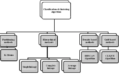
[image:1.595.311.556.440.593.2]

data clustering a significant challenge. Because of the high-speed processing requirements, many of the dynamic data clustering methods are extensions of simple algorithms such as k-means, modified to work in a dynamic data environment setting [4]. Numerous clustering algorithms have been developed in the literature, such as k-means, single linkage, and fuzzy clustering. A class of clustering algorithms based on the spectrum analysis of the affinity matrix has emerged as an effective clustering technique compared with the traditional algorithms, such as k-means or single linkage [5]. The following figure 1 shows the generalized classification of clustering algorithms.

Fig. 1. Classification of clustering algorithms.

Partitioning algorithms partitions the input data instances into disjoints spherical clusters. They are useful in application where each cluster represents a prototype, and other instances in the clusters are similar to these. In hierarchical methods, clusters which are very similar to each other are grouped into larger clusters. These larger clusters may further be grouped into still larger clusters. In essence, a hierarchy of clusters is produced. In density based methods, clusters are ‘grown’

(2)

starting with some data points and then including the other neighboring points as long as the neighborhood is sufficiently ‘dense’ [6]. These methods can find clusters of arbitrary shape and are useful in applications where such a feature is desired. In grid based methods the space of instances is divided into a grid structure. Clustering techniques are then applied using cells of the grid as the basic units instead of individual data points. This has the advantage of improving the processing time significantly.

II. PARTITIONING BASED CLUSTERING METHODS

K-means [7] is one of the simplest unsupervised learning algorithms that solve the well known clustering problem. The procedure follows a simple and easy way to classify a given data set through a certain number of clusters (assume k clusters) fixed a priori. The main idea is to define k centroids, one for each cluster. These centroids should be placed in a cunning way because of different location causes different result. So, the better choice is to place them as much as possible far away from each other. The next step is to take each point belonging to a given data set and associate it to the nearest centroid. When no point is pending, the first step is completed and an early grouping is done. At this point it is needed to re-calculate k new centroids as centers of the clusters resulting from the previous step. After having these k new centroids, a new binding has to be done between the same data set points and the nearest new centroid. A loop has been generated. As a result of this loop one can notice that the k centroids change their location step by step until no more changes are done. In other words centroids do not move any more. Finally, this algorithm aims at minimizing an objective

function, in this case a squared error function. The objective

function is described as

2

1 1 )

( _||

||

∑ ∑

= =

− =

k

j n

i

j j

i c

x J

where,

||

x

_i(j)

−

c

_j

||

2 is a chosen distance measure between a data point

x

_i(j)and the cluster centre

c

_j, is an indicator of the distance of the n data points from their respective cluster centers. The algorithm is composed of the following steps:

1. Place K points into the space represented by the objects that are being clustered. These points represent initial group centroids.

2. Assign each object to the group that has the closest centroid.

3. When all objects have been assigned, recalculate the positions of the k centroids.

4. Repeat steps 2 and 3 until the centroids no longer move. This produces a separation of the objects into groups from which the metric to be minimized can be calculated.

Although it can be proved that the procedure will always terminate, the k-means algorithm does not necessarily find the most optimal configuration, corresponding to the global

objective function minimum. The algorithm is also significantly sensitive to the initial randomly selected cluster centers. The k-means algorithm can be run multiple times to reduce this effect. K-means is a simple algorithm that has been adapted to many problem domains. It is a good candidate for extension to work with fuzzy feature vectors

III. HIERARCHICAL CLUSTERING

A. Single Linkage Clustering Algorithm

Single-linkage [8] clustering is one of several methods of agglomerative hierarchical clustering. In the beginning of the process, each element is in a cluster of its own. The clusters are then sequentially combined into larger clusters, until all elements end up being in the same cluster. At each step, the two clusters separated by the shortest distance are combined. The definition of 'shortest distance' is what differentiates between the different agglomerative clustering methods. In single-linkage clustering, the link between two clusters is made by a single element pair, namely those two elements (one in each cluster) that are closest to each other. The shortest of these links that remains at any step causes the fusion of the two clusters whose elements are involved. The method is also known as nearest neighbor clustering. The single linkage algorithm is composed of the following steps:

1. Begin with the disjoint clustering having level L(0) = 0 and sequence number m = 0.

2. Find the most similar pair of clusters in the current clustering, say pair (r), (s), according to d[(r), (s)] = min d[(i), (j)] where the minimum is over all pairs of clusters in the current clustering.

3. Increment the sequence number: m = m + 1. Merge clusters (r) and (s) into a single cluster to form the next clustering m. Set the level of this clustering to L(m) = d[(r), (s)].

4. Update the proximity matrix, D, by deleting the rows and columns corresponding to clusters (r) and (s) and adding a row and column corresponding to the newly formed cluster. The proximity between the new cluster, denoted (r, s) and old cluster (k) is defined as d[(k), (r, s)] = min d[(k), (r)], d[(k), (s)].

5. If all objects are in one cluster, stop. Else, go to step 2. The terms used in the above algorithm are explained in following section.

B. Complete Linkage Clustering Algorithm

(3)

in each cluster) that are farthest away from each other. The shortest of these links that remains at any step causes the fusion of the two clusters whose elements are involved. The method is also known as farthest neighbor clustering. The result of the clustering can be visualized as a dendrogram, which shows the sequence of cluster fusion and the distance at which each fusion took place. Mathematically, the complete linkage function — the distance D (X, Y) between clusters X and Y — is described by the following expression:

) , ( min ) , (

, d x y

Y X D

Y y X

x∈ ∈

=

where, D (X, Y) is the distance between elements x ε X and y

ε Y, X and Y are two sets of elements (clusters).

Complete linkage clustering avoids a drawback of the alternative single linkage method - the so-called chaining phenomenon, where clusters formed via single linkage clustering may be forced together due to single elements being close to each other, even though many of the elements in each cluster may be very distant to each other. Complete linkage tends to find compact clusters of approximately equal diameters.

The following algorithm is an agglomerative scheme that erases rows and columns in a proximity matrix as old clusters are merged into new ones. The N x N proximity matrix D

contains all distances d (i, j). The clustering are assigned sequence numbers 0, 1, ..., (n− 1) and L(k) is the level of the kth clustering. A cluster with sequence number m is denoted (m) and the proximity between clusters (r) and (s) is denoted

d[(r), (s)]. The algorithm is composed of the following steps: 1. Begin with the disjoint clustering having level L(0) = 0

and sequence number m = 0.

2. Find the most similar pair of clusters in the current clustering, say pair (r), (s), according to d [(r), (s)] = max d [(i), (j)] where the maximum is over all pairs of clusters in the current clustering.

3. Increment the sequence number: m = m + 1. Merge clusters (r) and (s) into a single cluster to form the next clustering m. Set the level of this clustering to L(m) = d[(r),(s)].

4. Update the proximity matrix, D, by deleting the rows and columns corresponding to clusters (r) and (s) and adding a row and column corresponding to the newly formed cluster. The proximity between the new cluster, denoted (r, s) and old cluster (k) is defined as d[(k), (r, s)] = max d[(k), (r)], d[(k), (s)].

5. If all objects are in one cluster, stop. Else, go to step 2.

C. Average Linkage Clustering Algorithm

Average-linkage clustering [10] merges in each iteration the pair of clusters with the highest cohesion. If data points are represented as normalized vectors in a Euclidean space, the cohesion G of a cluster C can be defined as the average dot product:

) ) ( ( )] 1 ( [

1 )

( C n

n n C

G −

−

= γ

where n =|C|,

γ

(C) =

∑

v

∑

w

<

v

w

>

C C

,

and

<

v

,

w

>

is

the dot product of v and w.

If an array of cluster centroids p(C) is maintained, where p(C) =

∑

v

<

v

>

C

, for the currently active clusters, then

γ

of the merger of C1 and C2, and hence its cohesion, can be computed recursively as

γ

(C1+C2) =

∑

<

>

+ +

w

v

w

v

C C C C

,

2 1 2 1

=

∑

<

>

∑

<

>

+ +

w

v

C C C

C1 2 1 2

=

<

p

(

c

1

+

c

2

)

>

Based on this recursive computation of cohesion, the time complexity of average-link clustering is O (n2log n). Firstly all n2 similarities for the singleton clusters are computed, and sort them for each cluster (time: O (n2log n)). In each of O (n) merge iterations, the pair of clusters with the highest cohesion in O(n) is identified; merge the pair; and update cluster centroids, gammas and cohesions of the O(n) possible mergers of the just created cluster with the remaining clusters. For each cluster, the sorted list of merge candidates is also updated by deleting the two just merged clusters and inserting its cohesion with the just created cluster. Each iteration thus takes O(n log n). Overall time complexity is then O (n2log n).

Note that computing cluster centroids, gammas and cohesions will take time linear in the number of unique terms T in the document collection in the worst case. In contrast, complete-linkage clustering is bounded by the maximum document length Dmax (if computed similarity using the cosine

for data points represented as vectors). So complete-linkage clustering is O(n2log n Dmax) whereas average-link clustering

is O(n2log n T). This means that usually it is needed to employ some form of dimensionality reduction for efficient average-linkage clustering. Also, there is only O (n2) pair wise similarities in complete-linkage clustering since the similarity between two clusters is ultimately the similarity between two vectors. In average-linkage clustering, every subset of vectors can have a different cohesion, so all possible cluster-cluster similarities cannot be computed.

IV. HIERARCHY BASED BALANCED ITERATIVE REDUCING AND

CLUSTERING

(4)

single scan of the database. In addition, BIRCH also claims to be the "first clustering algorithm proposed in the database area to handle 'noise' (data points that are not part of the underlying pattern) effectively".

Given a set of N d-dimensional data points, the clustering

feature CF of the set is defined as the

tripleCF =(N,LS,SS), where

LS

is the linear sum and

SS

is the square sum of data points. Clustering features are organized in a CF tree, which is a height with two parameters: branching factor B and thresholdT . Each non-leaf node contains at most B entries of the form[CF_i,child_i], where

child

_iis a pointer to its ith child node and

CF

_ithe clustering feature representing the associated sub cluster. A leaf node contains at most

L

entries each of the form

[

CF

_i

]

. It also has two pointers prev and next which are used to chain all leaf nodes together. The tree size depends on the parameterT. A node is required to fit in a page of size P. B and

L

are determined by P. So P can be varied for performance factor. It is a very compact representation of the dataset because each entry in a leaf node is not a single data point but a sub cluster. The algorithm consists of following steps.

1. Scans all data and builds an initial memory CF tree using the given amount of memory.

2. It scans all the leaf entries in the initial CF tree to rebuild a smaller CF tree, while removing outliers and grouping crowded sub clusters into larger ones.

3. There is an existing clustering algorithm is used to cluster all leaf entries. Here an agglomerative hierarchical clustering algorithm is applied directly to the sub clusters represented by their CF vectors. It also provides the flexibility of allowing the user to specify either the desired number of clusters or the desired diameter threshold for clusters. After this step a set of clusters is obtained that captures major distribution pattern in the data. However there might exist minor and localized inaccuracies which can be handled by an optional step 4.

4. The centroids of the clusters produced in step 3 are used as seeds and redistribute the data points to its closest seeds to obtain a new set of clusters. Step 4 also provides us with an option of discarding outliers. That is a point which is too far from its closest seed can be treated as an outlier.

In BIRCH each clustering decision is made without scanning all data point and currently existing clusters. It exploits the observation that data space is not usually uniformly occupied and not every data point is equally important. It makes full use of available memory to derive the finest possible sub-clusters while minimizing input output costs. It is also an incremental method that does not require the whole data set in advance.It makes a large clustering problem tractable by concentrating on densely occupied portions, and using a compact summary. It utilizes measurements that capture the natural closeness of data. These measurements can be stored and updated

[image:4.595.304.560.114.718.2]

incrementally in a height balanced tree. BIRCH can work with any given amount of memory. Following table I show the datasets that can be utilized to carry out data mining experimentations.

TABLE I. AVAILABLE DATASETS [9,4]

Datasets Properties

Number of Objects Number of Attributes

Car 1728 6

Iris 150 4

WDBS 569 30

Yeast 1484 8

Wine 178 13

Glass 215 9

Diabetics 768 8 Optical

Digits

5620 64

Musk 7074 167

TABLE II. COMPARATIVE ANALYSIS OF MOST COMMONLY USED

CLUSTERING ALGORITHMS

Algorithms Features Time

Complexity Limitations

Single

linkage Versatile Chaining Effect Complete

linkage

Tends to find

compact clusters --

Average linkage

Ranked well in evaluation

studies

It may cause elongated clusters

to split and for portions of neighboring elongated clusters

to merge

K-means

With a large number of variables, K-Means may be computationally

faster than hierarchical clustering (if K is

small)

Does not work well with non-globular

clusters

DBSCAN [10]

Can be used with databases that can accelerate region queries

Can’t cluster dataset well with large

differences in densities CLIQUE

[12]

Improves the Processing time

Significantly

(5)

The comparative analyses of the reviewed algorithms are given in the table II. In table II k – highest dimensionality, m- number of input points and C-number of clusters.

V. CONCLUSION AND FUTURE SCOPE

This paper presents the basic classification of clustering algorithms. The comparison of k-means, single linkage, average linkage, complete linkage, BIRCH, DBSCAN and CLIQUE is given in this paper on the basis of some basic parameters. The available datasets that researchers can utilize to carry out the research in data mining and clustering domain are listed in this paper. In the near future, the researchers can explore more reasonable ways of increasing the threshold dynamically, the dynamic adjustment of outlier criteria, more accurate quality measurements, and data parameters that are good indicators of how well any clustering algorithm is likely to perform.

REFERENCES

[1] Y. S. Lin, J. Y. Jiang and S. J. Lee, “A Similarity Measure for Text Classification and Clustering,” IEEE Trans. on Knowledge and Data Engineering, Vol. 26, No. 7, Jul 2014.

[2] Q. Zhao and P. Franti, “Centroid Ratio for a Pairwise Random Swap Clustering Algorithm,” IEEE Trans. on Knowledge and Data Engineering, Vol. 26, No. 5, Jul 2014.

[3] M. T. Mills and N. G. Bourbakis, “Graph-Based Methods for Natural Language Processing and Understanding – A Survey and Analysis,”

IEEE Trans on Systems, Man and Cybernetics: Systems, Vol. 44, No. 1, Jan 2014.

[4] M. Yuwono, S. W. Su, B. D. Moulton and H. T. Nguyen, “Data Clustering Using Variants of Rapid Centroid Estimation,” IEEE Trans on Evolutionary Computation, Vol. 18, No. 3, Jun 2014.

[5] D. Niu, J. G. Dy and M. I. Jordan, “Iterative Discovery of Multiple Alternative Clustering Views,” IEEE Trans on Pattern Analysis and Machine Intelligence, Vol. 36, No. 7, Jul 2014.

[6] M. A. Balaguer and C. M. Williams, “Hierarchical Modularization Of Biochemical Pathways Using Fuzzy-C Means Clustering,” IEEE Trans on Cybernetics, Vol. 44, No. 8, Jan 2014.

[7] S. Chen and C. Lui, “Clustering-Based Discriminant Analysis for Eye Detection,” IEEE Trans on Image Processing, Vol. 23, No. 4, Apr 2014. [8] A. Faktor and M. Irani, “Clustering by Composition”—Unsupervised

Discovery of Image Categories,” IEEE Trans. on Pattern Analysis and Machine Intelligince, Vol. 36, No. 6, Jun 2014.

[9] L. Sun and L. Guo, “Incremental Affinity Propagation Clustering Based on Message Passing,” IEEE Trans. on Knowledge and Data Engineering, Vol. 26, No. 9, Jul 2014.

[10] J. Gudmundsson and N. Valladares, “A GPU approach to subtrajectory clustering using the Frechet distance,” IEEE Trans on Parallel and Distributed Systems, Vol. 28, No. 9, Jan 2014.

[11] Q. Wu, Y. Ye, H. Zhang, T. Chow and S. Ho, “ML-TREE: A Tree-Structure-Based Approach to Multilabel Learning,” IEEE Trans on Nueral Networks and Learning Systems.