VERTICAL PRICE TRANSMISSION IN CHILI MARKET IN
INDONESIA
MAIKA FITRIANA
GRADUATE SCHOOL
BOGOR AGRICULTURAL UNIVERSITY
BOGOR
STATEMENT OF THESIS, SOURCE OF INFORMATION
AND COPYRIGHT
I hereby declare that thesis titled Vertical Price Transmission in Chili Market in Indonesia, was independently composed by me under the advisory committee supervision and has not been submitted to any other universities. Source of information derived or quoted from works published and unpublished from other writers have been mentioned in the text and listed in the bibliography at the end of this thesis.
I hereby assign the copyright of my thesis to the Bogor Agricultural University.
Bogor, March 2016
Maika Fitriana
SUMMARY
MAIKA FITRIANA. Vertical Price Transmission in Chili Market in Indonesia. Supervised by SUHARNO, SITI JAHROH, STEPHAN von CRAMON.
Like most developing countries, the agriculture sector contributes significantly to the Indonesian economy. In the Indonesian market, the vegetable sector is particularly important. Globally, Indonesia is the fifth of chili producing country in the world, next to China, Mexico, Turkey and Spain. Chili is an essential spice in the Indonesians diet. Chili production has received considerable attention in Indonesia due to extensive price fluctuations and its effect on inflation.
This paper examines the cointegration of chili prices between market players in the Indonesian chili market at three levels: farmer to trader (I), farmer to consumer (II), and trade to consumer (III). An error correction model was employed to measure the price transmission between different actors in the vertical market. The empirical results show that a long-run relationship exists at the farmer-trader, the farmer-consumer, and the trader-consumer levels. Moreover, in the short-run, price transmission between the market levels in the same city (I) is more rapid, and the price transmission between the direct market levels (I) is more rapid than the non-direct market level (II, III).
Price determination in the farm market is strongly influenced by seasonal chili production. The high production in the rainy season and low production in the dry season create high volatility of producer price (farmer). There are no arrangements on cropping patterns, so most farmers grow chili together simultaneously during the rainy season. Meanwhile in the dry season, not all farmers grow chili due to the limitation of water. There has no new technology to grow chili in the dry season or in dry land which can produce chili as good as in the rainy season and can be applied massively. Farmers have to buy water or build some irrigations by build well (ground water) so they can grow their chili in the dry season.
Over supply chili in the rainy season will lower chili price at the farmer level, but then if there is lack of supply chili price will be higher. Some big manufactured company or big chili sauce producers try to stabilize the price by using contract price. They block the seasonal price effects transmitted to retailer price or consumers. They have ability to storing chili for the stocks then manage the supply to provide stable supply in input for their product (output). The high price volatility of farm gate price inhibits the price transmission along the chili market chain. Therefore, the policy implication based on this factor is that the government should manage the price stabilization for farm gate price through overcome the unstable supply along the year.
RINGKASAN
MAIKA FITRIANA. Transmisi Harga Vertikal di Pasar Cabai di Indonesia. Dibimbing oleh: SUHARNO, SITI JAHROH, STEPHAN von CRAMON.
Seperti kebanyakan negara berkembang, sektor pertanian memberikan kontribusi yang signifikan terhadap perekonomian Indonesia. Di pasar Indonesia, sektor sayur sangat penting. Secara global, Indonesia merupakan Negara kelima penghasil cabai di dunia, bersama dengan China, Meksiko, Turki dan Spanyol. Cabai merupakan rempah-rempah penting dalam diet orang Indonesia. Orang Indonesia mengkonsumsi cabai pada tingkat 1,5 kg per kapita per tahun. Produksi cabai telah menerima banyak perhatian di Indonesia karena fluktuasi harga yang luas dan efeknya pada inflasi.
Studi ini membahas kointegrasi harga cabai antara pelaku pasar di Indonesia pada tiga tingkatan: petani kepada pedagang, petani kepada konsumen, dan pedagang kepada konsumen. Model koreksi kesalahan digunakan untuk mengukur transmisi harga antara aktor yang berbeda di pasar vertikal. Hasil empiris menunjukkan bahwa hubungan jangka panjang ada di petani-pedagang, petani-konsumen, dan tingkat pedagang-konsumen. Selain itu, dalam jangka pendek, transmisi harga antara tingkat pasar di kota yang sama lebih cepat, dan transmisi harga antara tingkat pasar langsung lebih cepat daripada tingkat pasar tidak langsung.
Harga cabai di tingkat petani sangat dipengaruhi oleh produksi cabai musiman. Produksi yang tinggi pada musim hujan dan produksi rendah di musim kemarau membuat volatilitas tinggi pada harga ditingkat petani. Tidak ada pengaturan pola tanam, sehingga sebagian besar petani menanam cabai bersama-sama secara berbersama-samaan selama musim hujan. Sementara itu di musim kemarau, tidak semua petani menanam cabai karena keterbatasan air. Belum ada teknologi baru untuk menanam cabai pada musim kemarau atau di lahan kering yang dapat menghasilkan cabai sebaik di musim hujan dan dapat diterapkan secara besar-besaran. Petani harus membeli air atau membangun irigasi dengan membangun sumur bor (air tanah) sehingga mereka dapat menanam cabai mereka di musim kemarau.
Kelebihan pasokan cabai (over supply) akan menurunkan harga cabai di tingkat petani, tapi kemudian pada saat kurang pasokan harga cabai akan lebih tinggi. Beberapa perusahaan manufaktur yang besar (produsen sambal) mencoba untuk menstabilkan harga ini dengan menggunakan harga kontrak. Mereka memiliki kemampuan untuk menyimpan cabai untuk stok untuk persediaan pasokan yang stabil untuk membuat produk mereka (output). Volatilitas harga yang tinggi pada harga produsen menghambat transmisi harga sepanjang rantai pasar (market chain). Oleh karena itu, implikasi kebijakan berdasarkan faktor ini adalah bahwa pemerintah harus mengelola stabilisasi harga untuk harga produsen dengan mengelola pasokan agar stabil sepanjang tahun.
© All Rights Reserved by Bogor Agricultural University, 2016
Copyright Reserved
It is prohibited to quote part or all of this paper without including or citing the source. Quotations are only for purposes of education, research, scientific writing, preparation of reports, critics, or review an issue; and those are not detrimental to the interest of the Bogor Agricultural University.
VERTICAL PRICE TRANSMISSION IN CHILI MARKET IN
INDONESIA
MAIKA FITRIANA
Master Thesis
as one of requirements to obtain a degree of Master Science
in
an Agribusiness Study Program
GRADUATE SCHOOL
BOGOR AGRICULTURAL UNIVERSITY
BOGOR
External Examiners Commission on the Exams Thesis: Dr Ir Harianto, MS
Thesis Title : Vertical Price Transmission in Chili Market in Indonesia
Name : Maika Fitriana
Student ID : H351120191
Approved Advisory Committee
Dr Ir Suharno, MADev Dr Siti Jahroh, BSc, MSc
Chairman Member
Aggred by
Head of Agribusiness Study Program Dean of Graduate School
Prof Dr Ir Rita Nurmalina, MS Dr Ir Dahrul Syah, MScAgr
ACKNOWLEDGMENT
All praise to God, The Gracious and The Merciful, for Allah blessings from the first until the last step of the research process. This research would have been impossible without the support from many people. I would like to appreciate everything they have given to me.
I would like to thank my supervisors Dr Ir Suharno MADev and Dr Siti Jahroh, BSc, Msc from Bogor Agricultural University, for their suggestions and valuable comments on this research from the beginning until the last step. Dr Ir Anna Fariyanti, MSi for valuable comment and evaluation in my colloquium. Prof Stephan von Cramon-Taubadel my supervisor in Goettingen University Germany, who support me academically. Dr. Ir. Harianto, MS and Dr. Amzul Rifin, SP MA, my examiners, who give valuable comments and support. I would like to acknowledge Prof Dr Rita Nurmalina, MS as the head of Master Science of Agribusiness concerning the double degree program between IPB and Master of International Agribusiness Goettingen University.
I would like to acknowledge the support from the Ministry of Education of Indonesia (DIKTI) for funding my study in Germany. Dede Arnanto, SE, MSi staff of Ministry of Trade of Indonesia for provided me time series data of chili price. Mr. Saeran for his valuable comments and for provided me chili price in farm gate price and trader price in Banyuwangi.
My sincere thanks to Ms. Grete Thinggaard, academic adviser in Goettingen University. My sincere thanks to Ms. Yuni and Ms. Dewi, who are staff of Master Sscience of Agribusiness IPB.
My sincere thanks to all my friends in Magister Science of Agribusiness IPB as well as in SIA program-Goettingen University, Ka Majek, Mas Angga, Mba Intan, Mba Wida, Ica, Dhea, Rizah, Irfan and Ian for a friendly and warm environment during my study. I dedicate this work to my beloved parents, and my little brother who always give me their pray, love, and never ending support and encouragement for me.
Bogor, March 2016
LIST OF TABLES
1. Chili harvested by area (ha) and region in Indonesia, 2009-2013 4
2. Indonesian chili production by region, 2009-2013 5
3. Descriptive analysis of Indonesian chili prices, 2009-2013 10
4. Descriptive analysis of the farmer, trader, and consumer prices of
Indonesian chili, 2009-2013 17
5. Results of the ADF-test for chili prices at the farmer level, trader level and
consumer level 19
6. Results of Johansen trace test for chili prices at the farmer level, trader
level and consumer level 20
7. Results of Granger-Causality test for chili prices at the farmer level, trader
level and consumer level 21
8. Error correction model of chili prices between farmer and trader prices 22
9. Error correction model of chili prices between farmer and consumer 23
10. Error correction model of chili prices between trader and consumer 24
LIST OF FIGURES
1. Vegetable Production (MT) in Indonesia, 2013 1
2. Production and yield of chili in Indonesia, 2009-2013 4
3. Indonesian chili production by seasons 5
4. Annual chili consumption in Indonesia per capita 6
5. Monthly export of chili from Indonesia in 2013 7
6. Indonesian chili import per month, 2013 7
7. Market supply chain of chili in East Java, Indonesia 8
8. National consumer price for Indonesian chili, 2009-2013 9
9. Daily farmer, trader and consumer prices for Indonesian Chili, 2009-2013
17
10. Plot series of logarithmic prices of Indonesian chili at the farmer level,
2009-2013 18
11. Plot series of logarithmic prices of Indonesian chili at the trader level,
x
12. Plot series of logarithmic prices of Indonesian chili at the consumer level,
2009-2013 19
LIST OF APPENDICES
1. Chili harvested by area (ha) and province in Indonesia, 2009-2013 2. Production of chili by province in Indonesia, 2009-2013
3. Yield of Chili by Province in Indonesia, 2009-2013 4. Output of ADF-test for Pfarmer_log
5. Output of ADF-test for Ptrader_log 6. Output of ADF-test for Pconsumer_log 7. Output of ADF-test for Pfarmer_log_d1 8. Output of ADF-test for Ptrader_log_d1 9. Output of ADF-test for Pconsumer_log_d1
10.Output of Johansen trace test for chili prices in farmer level and trader level
11.Output of Johansen trace test for chili prices in farmer level and consumer level
12.Output of Johansen trace test for chili prices in trader level and consumer level
13.Output of Granger causality test for chili prices in farmer level and trader level
14.Output of Granger causality test for chili prices in farmer level and consumer level
15.Output of Granger causality test for chili prices in trader level and consumer level
16.Output of VECM for Pfarmer_log and Ptrader_log 17.Output of VECM for Pfarmer_log and Pconsumer_log 18.Output of VECM for Ptrader_log and Pconsumer_log
19.Chili intercropped with rubber plantation, Banyuwangi, East Java 20.Chili field on irrigated land
21.Sortation of chili is done by the trader’s workers
22.Chili packaging using carton box (30 kg), done by chili trader
LIST OF ABBREVIATIONS
ADF : Augmented Dickey-Fuller
APT : Asymmetric price transmission
AVRDC : Asian Vegetable Research Development Center
BAPPENAS : Badan Perencanaan Pembangunan Nasional; National Development Planning Agency
BPS : Badan Pusat Statistik; Statistics Indonesia
Deptan : Departemen Pertanian. Department of Agricultural the
Indonesian Ministry of Agriculture DGH : Directorate General of Horticulture
ECM : Error correction model
IDR : Indonesia Rupiah
Kemendag Kementerian Perdagangan; Indonesian Ministry of Trade
MoA : Indonesian Ministry of Agriculture
UNCTA : United Nation Conference on Trade and Development
USD : United States Dollar
1 INTRODUCTION
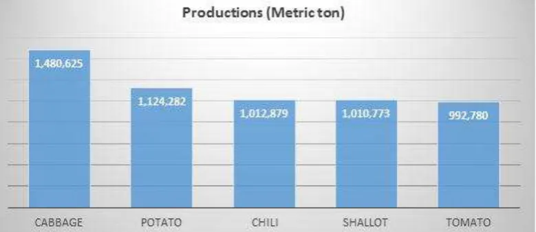
BackgroundLike most developing countries, the agriculture sector contributes significantly to the Indonesian economy. In the Indonesian market, the vegetable sector is particularly important. The five vegetables with the highest production are cabbage, potatoes, chili, shallot and tomatoes. Figure 1 shows the production quantity of vegetables in Indonesia. From the figure, we can see that chili was the third greatest contributor to vegetable production in 2013.
Figure 1. Vegetable Production (MT) in Indonesia, 2013
Source: Directorate General of Horticulture, Ministry of Agriculture (2014)
Globally, Indonesia is one of the top five chili producing countries in the world (UNCTAD, 2013), along with China, Mexico, Turkey and Spain. The top five chili exporters, however, are the Netherlands, Spain, Canada, the United States and France. Like most of the five leading chili producing countries, Indonesia is not a major exporter for this commodity; rather they dedicate their production to national consumption.
Chili is an essential spice in the Indonesians diet. The Indonesians consume chili at a rate of 1.5 kg per capita annually (Bappenas, 2013). The majority of Indonesians consume at least a small amount of chili every day. Therefore, as is the case with salt and many other condiments, the demand elasticity of chili is inelastic (Asian Vegetable Research Development Center, 2006).
2
Generally, the marketing channel of vegetables in Indonesia passes through from farmer to collector and local retailer. Then, distribution channel usually continue flows to wholesale markets and inter islands traders, and traditional retailers. Then, finally it is received by the consumer. However, the implementation of trade liberalization in 1990s, and the removal of restriction of the Foreign Direct Investment (FDI) in 1998 have stimulated the rapid growth of the supermarket sector in Indonesia. In short period, the sales of fresh vegetables in the supermarket increase rapidly. Then, it has led to a change of vegetables market chain where new channels are not only the supermarkets and food processing industries, but also farmer associations, hotels and restaurants have emerged in the marketing chain in Indonesia (Natawidjaja et al. 2007).
Over 60% of chili is produced on Java Island, with East Java being one of the most influential sources (White et al. 2007). Banyuwangi is a city that produces substantial quantities of chili in East Java. This paper will elaborating on the market in Banyuwangi, East Java, including an overview and analysis of prices incurred by farmers and traders. Moreover, the consumer price level that is considered in this study comes from Jakarta, where 90% of the chili is sold.
Problem Statement
Chili production has received considerable attention in Indonesia due to extensive price fluctuations and its effect on inflation (Saptana et al., 2012, Farid & Subekti, 2012). Additionally, chili is an important crop that is commonly produced by small-scale farmers. Furthermore, it has an important role as a source of cash flow and daily income for small-scale producers (Sahara et al., 2011).
Many recent studies focus on analyzing the disparity between markets to investigate price and market mechanisms. The chili market is in need of further study in order to understand the structure of its commodity chain, as well as its characteristics. Based on the description of chili market in Indonesia, several issues need to be further investigated by analyzing price transmission between different actors in the vertical chain:
1. How the vertical price transmission between farmer level and trader level? 2. How the vertical price transmission between farmer level and consumer
level?
Research Objectives
According to the description above, the objectives of this paper are:
1. To analyze the vertical price transmission between farmer level and trader level
1. As a reference and consideration in setting policy related to to chili price in Indonesia. Banyuwangi, trader in Banyuwangi, and consumen of chili in Jakarta. The scope of the discussion in this study includes price transmission investigated by analyzing between different actors in the vertical chain: farmer, trader, and consumer using VectorEerror Correction Model (VECM).
The limitations of this study are: (1) The source of data is limited to the data from farmer and trader in Banyuwangi, and price data of the consumer from Indonesian Ministry of Trade (2) The analysis of vertical price transmission is limited to red chili (cabe merah besar); and (3) Chili price data used in this study is daily time series from January 2009-December 2013.
2 LITERATURE REVIEW
National Production and ConsumptionIndonesian chili production is dominated by the production of chili on Java Island and Sumatera Island (White et al., 2007). Chili plants are mostly grown on small plots and is often considered to be a cash crop as it is a main crop in some areas (AVRDC, 2006), (Saptana et al., 2012). Chili plants are usually cultivated in paddy fields (irrigated or rainfed) and on dryland fields. On irrigated land, chili is typically planted after rice so that cropping patterns are influenced by the rice, and is therefore rely upon climatic conditions, especially rainfall.
4
metric tons in 2011, 954,312 metric tons in 2012, and 1,012,800 in 2013, leading to an average production growth of 6% during this five year time period.
The average chili yield, however, experienced slight decreases from 2010 to 2013, going from 6.72 metric tons per hectare to 6.58 metric tons per hectare. Despite this slight decrease, the trend of average yield from 2009 to 2013 showed increasing production. The national average yield for 2009-2013 was 7.35 metric tons per hectare. Both the national production volume and productivity are present in Figure 2.
Figure 2. Production and yield of chili in Indonesia, 2009-2013 Source: Ministry of Agriculture (2014), and Statistics Indonesia (2014)
On the other hand, the average yield across Indonesian provinces has a great deal of variation. Java Island has the highest yield with approximately 9.02 metric tons per hectare, with the second highest yields coming from Sumatera at 7.79 metric tons per hectare, with the other Indonesian islands averaging roughly 5.98 metric tons per hectare. Provincial data from Statistics Indonesia (BPS) and the Directorate General of Horticulture (DGH) of the Ministry of Agriculture are summarized in Tables 1 and 2, with all provincial data from 2009-2013 being available in Appendices 1-3.
Table 1. Chili harvested by area (ha) and region in Indonesia, 2009-2013
Region Harvested land area (ha) Average
(Ha)
Percentage
(%)
Growth
(%)
2009 2010 2011 2012 2013
Sumatera 47,943 52,952 51,403 49,677 52,528 50,900 42.07 2.48
Java 57,424 57,946 56,479 56,303 57,703 57,171 47.26 0.14
Others 11,811 11,857 13,181 13,845 13,879 12,914 10.67 4.21
Indonesia 117,178 122,755 121,063 119,825 124,110 120,986 100 1.48
The total harvested area for Indonesian chili from 2009 to 2013 was just 2009 to 2013, with an overall growth percentage of about 4%.
Table 2. Indonesian chili production by region, 2009-2013
The total chili production in Indonesia from 2009 to 2013 is presented in Table 2. Chili production in Indonesia has demonstrated an increasing trend over the five year period between 2009 and 2013. Java, Sumatera and other regions show a positive growth trend, with an average of 6.5%. Sumatera has the highest percentage of growth at approximately 9.5%, Java at 5.1% and other regions at about 7.3%. As previously mentioned, Java and Sumatera are the dominant chili producers in Indonesia accounting for nearly half of the total production.
Figure 3. Indonesian chili production by seasons Source: Webb & Kosasih (2011)
6
Figure 4. Annual chili consumption in Indonesia per capita Source: Ministry of Agriculture (2014)
Figure 4 presents the total consumption of chili in Indonesia. According to the Ministry of Agriculture (2014), the total chili consumption in Indonesia does experience fluctuations, with the average consumption, however, being about 1.5 kg per capita annually. This consumption value, however, is not always steady due to the unstable price of chili. In 2008, overall chili consumption decreased sharply, yet the average weight of consumption increased from the year before. As previously mentioned, the consumption of chili is inelastic. From the graph above, we can see that the price of chili does not have a dramatic effect on chili consumption.
There are no exact data on aggregate consumption of chili in Indonesia. However, the data of chili consumption per capita can be seen as a benchmark for the aggregate consumption of chili in Indonesia.
Export and Import
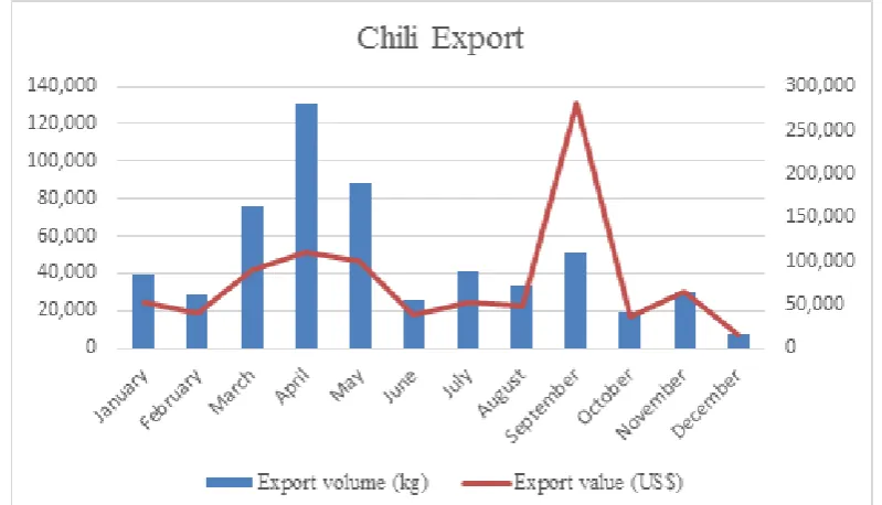
Figure 5. Monthly export of chili from Indonesia in 2013 Source: Export-import database (Ministry of Agriculture, 2014)
Here, we present monthly export data for chili in Indonesia in 2013 according to Ministry of Agriculture (2014). The total chili import for 2013 was 23,145 metric tons, valued at 27,525,616 USD. The total volume of chili import in Indonesia was forty times more than the total export in 2013. The primary sources
for Indonesia’s chili imports are India, China and Thailand. Figure 6 presents Indonesia’s monthly chili import in 2013.
8
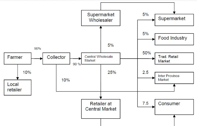
Marketing Channel
The market supply chain of chili in Indonesia differs by region, but some features remain constant throughout the country. We will use this marketing channel from White et al. (2007) for example. Chili marketing channel embraces link that happened between farms gate (producers) and final consumer. According
to Stern et al. (1996: 1), “marketing channels can be viewed as sets of
interdependent organizations involved in the process of making a product or
service available for consumption or use”. The chili market supply chain consists of the farmer, trader (collector), wholesaler, retailer, restaurant (food stall), and consumer. The chili marketing channel in East Java is illustrated in Figure 7.
Figure 7. Market supply chain of chili in East Java, Indonesia Source: White et al. (2007)
There are five common marketing options for Indonesian farmers (Shepherd & Schalke, 1995):
1. Farmers can go to the local market themselves, where they sell to traders who supply wholesale markets
2. Traders buy the entirety of the production field (standing crop purchase) and deliver to wholesale markets
3. Traders collect from farmers then deliver to wholesales markets 4. Trader buys from farmers and sells to the retail market
5. Farmers sell to a packing house
some farmers will choose this method to have guaranteed cash in hand. The standing crop buying method, however, is not common in the chili sector.
Typically, chili traders give credit for chili seed and fertilizer before the farmer beings planting. After harvest, the farmer will sell their output to the same trader that gave them credit. When the harvest time begins, farmers will go to the trader every day to sell their crop until the end of the harvesting period. By doing so, farmers ensure better access to credit, while traders reduce the risk of not obtaining enough product.
Another main actor in the market supply chain of chili is farmer associations. An important benefit of farmer associations is that they can sell chili to institutional buyers such as chili sauce companies, supermarkets and exporters. An Individual farmer cannot sell their chili directly to these organizations due to the small scale of the farmer; most farmers only produce a small amount of chili, and the quality of the product is not uniform.
Farmers do not sort their chili outputs before selling them to the trader. The trader will take care of the sorting process, based on color and physical condition, at an estimated cost of 500 IDR per kg (Webb et al., 2012). There is no storage cost at this stage because the entire chili output will be sent to another marketing channel within a day.
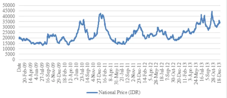
Prices in Indonesia
Chili prices in Indonesia have shown high fluctuations in between 2009 to 2013, as shown in Figure 8. A standard characteristic of chili prices in Indonesia is the extensive fluctuations, often the prices doubled in one month and then proceeded to decrease gradually.
10
Table 3 shows a comprehensive view of the descriptive analysis of the national consumer price of chili in Indonesia.
Source: Author’s calculations with data from the εinistry of Trade (2014)
Price volatility explains the variance of data compared to their mean. The price volatilities of food commodity are really important. Price volatility will influence economic and welfare of the society (Bustaman 2003). When chili prices increase, the composition of public expenditure on chili will increase. It will make reduction of revenue allocation for the other needs such as education and health. If the food prices increase continuously and volatile, the more onerous burden for society which can reduce the welfare of society.
Price stabilization on food can enhance economic growth and food security (Timmer 1996; Timmer 2004; and Dawe 2011). The advantages of price stabilization are that it can reduce the level of risk faced by producer and stimulates farmers to invest more to produce and raise productivity, meanwhile for consumer can get benefit from stable price and can alleviate poverty. These notions assumed that food price transmitted completely from consumer to producer.
The price stabilization mechanism and its consequences are explained by simple Marshalian theory from Waugh-Oi-Massell in Newbery and Stiglitz (1981) (Istiqomah 2006). This theory assumes that the supply and demand are linear in the market and will response instantaneously when there is change of supply or demand, and additive stochastic disturbances. The changes of price equilibrium in the market due to supply or demand changes in the short-run will cause price volatility. The price stabilization is aimed to dampen the unstable prices and lead the prices to the mean of its prices.
As of yet, there is no comprehensive solution from the government regarding the fluctuations in the price of chili that has happened nearly every year. Some solutions from the government are monitoring supply, as well as the price of the chili by giving permission to the importers to buy chili from another country such as China, India and Thailand.
3 FRAMEWORK
Market Integrationhappens and all profitable arbitrage opportunities removed, prices are equalized up to the cost of commerce (Barrett, 2001). Market integration is a measure of the degree to which demand and supply are transmitted from one region to another region (Fackler & Goodwin, 2001). Similarly, Barrett and Li (2002) describe market integration as the core on trade of physical goods as tradability in the operation. Tradability means transferring information when there is surplus of good in one market and/or there is opportunity of physical flow of goods.
Besides linked to flow of physical goods, the concept of market integration also refer to co-movement of price between markets indicated by LOP. As define by Fackler & Goodwin (2001), strong LOP hold when spatial arbitrage condition as an equality between spatial markets. An integrated market exists when connected markets display high price correlations. If trade takes place beetwen different markets for homogenous goods, the price in the origin market (Pi) is LOP, a temporary price disparity between markets will arise, but it will gradually return to equilibrium in the long run (Fackler & Goodwin, 2001). The concept of LOP expects that all information in the markets is obtainable so that optimal arbitrage and no-barriers to trade can be implemented (McNew, 1996), (Jensen, 2007). However, some literature suggests that this expectation is too idealistic and would never happen in practice.The concept of LOP expects that all information in the markets is acquired to implement optimal arbitrage and no-barriers to trade (McNew, 1996), (Jensen, 2007). However, some literature suggests that this expectation is too idealistic and would never happen in practice.
It is possible to have market integration despite being in a no-trade between markets situation, as long as they are part of the marketing system. Market integration is not automatically a reference to market competitiveness (Fackler & Goodwin, 2001). In the same sense, there is possibility of a no-market integration situation in the case of physical arbitrage where this absence of market integration exists when there is market segmentation (Barrett & Li, 2002). The absence of trade may also suggest that markets are in spatial equilibrium (Stephens et al., 2012).
12
Price Transmission in Vertical Food Chain
Vertical price transmission is identified by the magnitude and speed of adjustment of goods that pass through the supply chain and are developed at any other level of the marketing process (Vavra & Goodwin, 2005). Magnitude is defined as the size of the effect that has been transferred to another level of the market. It also indicates the size of the response to each market level due to the extent of the impact (change) which appears at another level of the market. On other hand, speed implies the significant lags of adjustment. The size of the effects is typically of the most interest; still, the speed of adjustment is essential to fully understanding the integration. The speed with which a market adjusts to change (shock) from another market is specified by the actions of market agents who are engaged in the transactions.
As a change in prices could determine the magnitude and speed of adjustment cost, then asymmetric price transmission (APT) becomes an important concept. Under asymmetric price transmission, producers and/or consumers may not benefit if there is an increase or decrease in the price of goods in another level of the market. A common occurrence is when the price increases at the retail
Previous Study
Many studies have been done to examine price transmission and market integration of staple food commodities in Indonesia, relatively few studies, however examine market integration and price transmission with respect to the vegetables market. A study by Jubaedah (2013)regarding market integration of the red chili commodity in Indonesia focuses on spatial price transmission and market integrations between wholesale markets in Jakarta and 23 producer markets throughout Indonesia. Findings indicate the potential factors behind either lacking or strong market integration in the Indonesian chili market. The quality of infrastructure, distance between markets, and the size of the market tend to affect the integration on the markets. With these findings, Jubaedah gives a couple policy recommendations with the aim of achieving better market integration in the Indonesian chili sector; first, improve the development of infrastructure to minimize transfer costs. Second, develop the marketing information system within the country in order to gain clear insight into chili price and improved marketing information.
Webb et al. (2012) study the relationship between chili traders and price
volatility. Their research question, “Do chili traders make price volatility worse?”
led to the conclusion that chili traders are relatively good about responding to a price shock by quickly transferring chili to other parts of the island. However, chili traders do not have stocks to anticipate increasing demand shocks in the chili sector, which may be potentially harmful when dealing with volatile prices. Two policies are suggested by Webb et al., one is to permit imports of fresh chili from other countries, and the second is to subsidize investment in cold storage, which can help holding stocks to reduce the chili price fluctuations.
Farid and Subekti (2012) examined production, consumption, distribution and price dynamics of chili production in Indonesia. From this research, it is made apparent that there are factors that can lead to price disparities for chili price across the country. This is possibly due to the large concentration of chili production taking place in Java and Sumatera, despite all Indonesian people consuming chili. Not all provinces can produce chili, thus leading to the conclusion that poor infrastructure and high transfer costs can often lead to price disparities. This research also findings the factors that influenced the price of chili in Indonesia; 1) Planting pattern (the production of chili), 2) Cost of production (seed and fertilizer), 3) Distribution of chili; not all the provinces in Indonesia can meet the needs of chili consumption, and non-Java region have bad infrastructures, 4) Consumption when there is Ramadhan and Idul Fitri festival. As with Jubaedah and Webb et al., this paper indicates policy recommendations, the most relevant being to improve some infrastructure within the country.
Hypotheses
1. Price transmission is more rapid between the farmer-trader level than between the farmer-consumer level.
14
3. Price transmission is more rapid between the trader-consumer level than between the farmer-consumer level.
4 RESEARCH METHODOLOGY
Data DescriptionThe present study uses daily consumer data of chili prices in Jakarta, trader prices in Banyuwangi, and farmer prices in Banyuwangi from January 2009 until December 2013. The data is secondary time series data taken from the Indonesian Ministry of Trade, Statistics Indonesia and Ministry of Agriculture. All of the time series data are transformed to logarithmic form.
All farmers price is a price that farmer get by selling their chili, all farmers price is collected by one trader. This trader buy chili from about 15 farmers a day. All trader price is a price that trader get by selling their chili to other traders within kabupaten (district). Trader price is collected daily using their own record book. This trader usually sell their chili to three traders based on price.
Price Transmission Analysis
Price transmission analysis is used to answer the research questions of vertical market integration and vertical price transmission of farmer level price in Banyuwangi, trader level price in Banyuwangi and consumer price in Jakarta. The data was run using STATA version 13.0 statistical software for the following statistical tests: 1) Unit root test for stationarity, 2) Johansen test for cointegration, and 3) Granger-causality test for testing direction of price transmission (causality). The next step is to model the vertical price transmission in accordance with the following classifications: 1) price transmission between the farmer level and trader level, 2) price transmission between the farmer level and consumer level, and 3) price transmission between trader level and consumer level. This study applies the standard linear error correction model (ECM) for data estimation.
Unit Root Test
To examine whether the data is stationary or not, we use the unit root test. The stationarity of each data series is needed to detect the presence of spurious regression in the model. A spurious regression will indicate that the result of the regression may not have a direct causal relation, but it is possible that they do. This paper used an Augmented Dickey-Fuller (ADF) test, which is an adjustment of the Dickey-Fuller (DF) test that is used to check the presence of unit root for each variable in the model. The ADF model can be estimated as follows:
Δ Yt= α0+ α1 T + tYt-i + Σ βiΔYt-i + t , ~ΠD (0, 2) (1)
If the null hypothesis of | t| = 0 is rejected, then the conclusion is that the
data series is stationary, where if the null hypothesis of | t| = 0 is accepted, then
the data series is not stationary.
Cointegration Test
The next step is the cointegration test, which tests for the presence of a
co-integrated relationship of two different market level’s price data. Cointegration of two market levels indicates that there is a tendency for the price to demonstrate one common behavior in the long run. If two price series in two markets are integrated in the same order, i.e., I (d), and there is a linear relationship between the price series’, then it can be assumed that those two markets are co-integrated.
The hypotheses of this test are:
cointegration test examines the presence of cointegrating vectors in the models at the farmer-trader price level, farmer-consumer price level and trader-consumer level.
Granger Causality Test
The Granger causality test examines the direction of the price transmission between the two market levels. If there are two price series, and one of the prices (Pit) current values are lagged, it can predict the value of another price (Pjt), then
Pit influence Pjt.
There are three categories of causality that may potentially take place: 1. No causality between two prices
2. Unidirectional causality; this occurs when there is only one direction of causality between prices, e.g., Pit can be predictive of Pjt,
but not the other way around
3. Bilateral causality (Reciprocal causality); this means that both prices can be predictive of each other.
Error Correction Model (ECM) Estimation
The third step is to create error correction models. The error correction term of ECM depicts the short-run adjustment of certain prices toward the long-run equilibrium. Meyer & von Cramon-Taubadel (2004) describe the error correction term through the following equation:
∆P1t = θ1 + αECTt-1 + ∑ 2i ∆ P1t-1 + ∑ 3j ∆P2t-j+ t (2) where α represents the percentage of the price adjustment in a certain period;∆P1t,
16
value θ1; changes in prices of the cointegration is indicated by ∆P2t-j; and the
distance of the variables in their last period is represented with ECTt-1.
5 RESULTS
Concept in Price DataThere are three level markets prices that used in this study; farm gate rices, wholesale prices, retail prices.
Farm Gate Prices
The farm gate prices are in principal the prices received by farmers for their produce at the location of farm. Thus the costs of transporting from the farm gate to the nearest market or first point of sale and market charges (if any) for selling the produce are, by definition, not included in the farm gate prices. Thus the prices collected from such markets may be adjusted for these costs to arrive at farm gate prices.
Trader Prices
After an agricultural product leaves the farm-gate, it may pass through one or even two wholesale markets and a chain of other "middlemen before reaching the retailer from whom the ultimate consumer buys it. This trader price that was used is a direct trader, who buy chili from farmers in same city, Banyuwangi.
Retail Prices
The price of a good or product when it is sold to the end user for consumption, not for resale through a third-party distribution channel.
Figure 9 shows where these three prices in marketing channel.
Figure 9. Three Variables Price for study
1 2
Note: 1. Farm gate prices, 2. trader prices, 3. Retail prices
These three level markets prices will be referred as : 1. Farm gate prices (farmer), 2. Trader prices (trader), 3. Retail prices (consumer)
Price Transmission Analysis
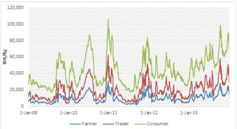
Figure 10 shows the monthly prices, in IDR/kg, of the three market levels in the vertical chain.
Figure 10. Daily farmer, trader and consumer prices for Indonesian Chili, 2009-2013
Source: Ministry of Trade (2014)
Table 4. Descriptive analysis of the farmer, trader, and consumer prices of Indonesian chili, 2009-2013
Variable Number of
observation
Mean (IDR)
Std. Dev.
C.V. Min.
(IDR)
Max. (IDR)
Farmer 1,304 9,666 5,395 0.558 1,750 31,000
Trader 1,304 10,204 5,584 0.547 2,000 32,000
Consumer 1,304 23,835 8,008 0.336 11,000 50,000
Source: Author’s calculations based on data from the Ministry of Trade (2014)
18
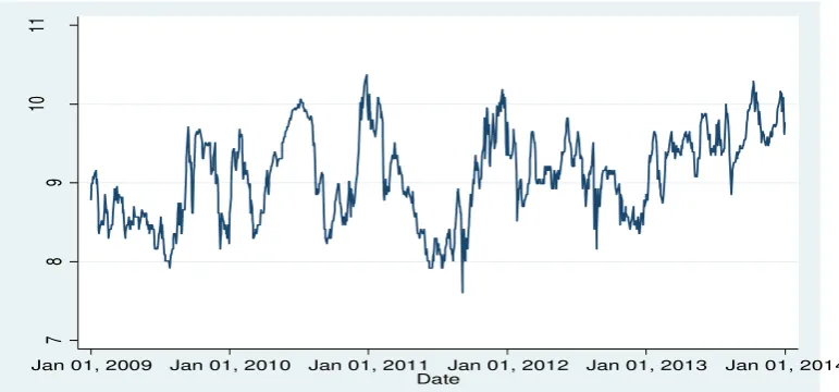
distributions less skewed. This transformation can also be valuable for both recognizing patterns in the data that can be easily interpreted and can help to meet the assumptions of inferential statistics. Figure 10-12 presents a plot series of prices at the farmer level, trader level and consumer level.
Figure 11. Plot series of logarithmic prices of Indonesian chili at the farmer level, 2009-2013
Source: Author’s representation based on data from the εinistry of Trade (2014)
Figure 12. Plot series of logarithmic prices of Indonesian chili at the trader level, 2009-2013
Source: Author’s representation based on data from εinistry of Trade (2014)
7
8
9
10
11
Jan 01, 2009 Jan 01, 2010 Jan 01, 2011 Jan 01, 2012 Jan 01, 2013 Jan 01, 2014
Date
7
8
9
10
11
Jan 01, 2009 Jan 01, 2010 Jan 01, 2011 Jan 01, 2012 Jan 01, 2013 Jan 01, 2014
Figure 13. Plot series of logarithmic prices of Indonesian chili at the consumer level, 2009-2013
Source: Author’s representation based on data from εinistry of Trade (2014)
Unit Root Test
Stationarity is an essential condition in the time series analysis to acquire unbiased estimations. In the present study, an ADF-test is used to check whether a unit root is present or not. When the data have no unit root, it indicates that the data are stationary. All price data in the three market levels are transformed into logarithmic form. As shown in Table 5, the absolute values of all of the variables are less than the absolute value of critical values at that particular level. This indicates that the null hypothesis of non-stationarity cannot be rejected at the ten percent significance level. For the first difference, we can reject the null hypothesis for non-stationarity at the one percent level of significance, meaning that all variables in first difference are stationary. Thus, we can conclude that all price variables in the model are not stationary at the level, but are stationary in the first difference. I(1)
A complete output of the ADF-test is available in Appendices 4-9.
Table 5. Results of the ADF-test for chili prices at the farmer level, trader level
Source: Author’s estimates; significance levels: 10% (*), 5% (**), 1% (***)
9
Jan 01, 2009 Jan 01, 2010 Jan 01, 2011 Jan 01, 2012 Jan 01, 2013 Jan 01, 2014
20
Cointegration Analysis
According to the result of the ADF-test, all of the variables integrated ~ I (1); therefore, it is necessary to proceed to the next step of the analysis by using the Johansen cointegration test. For this analysis, three pairs of variables were formed and tested. The null hypothesis is R = 0, indicating that there is no cointegraton in the relationship, were rejected at the five percent significance level for all three pairs of variables. The null hypothesis for R = 1, indicating that there is one case of cointegration in the relationship, cannot be rejected for all three pairs of price variables.
Table 6. Results of Johansen trace test for chili prices at the farmer level, trader level and consumer level
Variable Rank Trace statistic 5% Critical value
Farmer and Trader 0 115.345 12.53
1 0.005** 3.84
Farmer and Consumer 0 101.866 12.53
1 0.045** 3.84
Trader and Consumer 0 106.306 12.53
1 0.041** 3.84
Source: Auhor’s estimates, significance levels: 5% (**)
Granger Causality Test
Table 7. Results of Granger-Causality test for chili prices at the farmer level,
The results of error correction model between farmer and trader, as shown in Table 8. There is long run relationship between the farmer prices and the trader prices. As was estimated using Granger causality test, the causality goes from the farmer prices to trader prices. The estimation shows that in the long run, an increase (decrease) of one percent of chili price at the farmer level will lead to a increase (decrease) 0.976 percent of the trader prices.
22
Table 8. Error correction model of chili prices between farmer and trader prices
Variable Parameter Variable Parameter
∆Trader_log(t) ∆Farmer_log(t)
ect(t-1) -0.133* ect(t-1) 0.198*
∆Trader_log(t-1) -0.254 ∆Farmer_log(t-1) -0.100
∆Farmer_log(t-1) 0.337** ∆Trader_log(t-1) 0.196
Intercept 0.0006 Intercept 0.0004
Long Run
Trader_log(t-1)
Intercept 0.274
Pfarmer_log(t-1) 0.976***
Source: Author’s estimates, significance levels: 1% (***), 5% (**), 10% (*)
Trader and farmer have direct interaction in the trade. Here trader and farmer are in Banyuwangi. So they have strong linkage in product flow which is influence the price determination in both markets. The transaction costs factor between them are indicated to be relatively low, because the interactions are take place in one region. In these interactions there are value added by sortation and packaging make the price gap between trader and farmer
The results of error correction model between farmer and consumer, as shown in Table 9. There is long run relationship between the farmer prices and the consumer prices. As was estimated using Granger causality test, the causality goes from the farmer prices to consumer prices. The estimation shows that in the long run, an increase (decrease) of one percent of chili price at the farmer level will lead to an increase (decrease) 0.635 percent of the consumer prices.
Table 9. Error correction model of chili prices between farmer and consumer
Variable Parameter Variable Parameter
∆Consumer_log(t) ∆Farmer_log(t)
ect(t-1) -0.088*** ect(t-1) 0.040***
∆Consumer_log(t-1) 0.073*** ∆Farmer_log(t-1) 0.025
∆Pfarmer_log(t-1) -0.016 ∆Consumer_log(t-1) 0.122***
Intercept 0.0003 Intercept .0006
Long Run
Consumer_log(t-1)
Intercept 4.299
Farmer_log(t-1) 0.635***
Source: Author’s estimates, significance levels: 1% (***), 5% (**), 10% (*)
Farmer and consumer do not have direct interaction in the trade. Here Farmer are in Banyuwangi and consumer in Jakarta. So they do not have strong linkage in product flow which is influence the price determination in both markets. The transaction costs factor between them are indicated to be relatively high, because the interactions are take place in different region. In these interactions there are value added by sortation and packaging make the price gap higher than between trader and farmer. This interaction have the longest stage from the start of the chain until the end of the market chain (consumer).
The results of error correction model between trader and consumer, as shown in Table 10. There is long run relationship between the trader prices and the consumer prices. As was estimated using Granger causality test, the causality goes from the trader prices to consumer prices. The estimation shows that in the long run, an increase (decrease) of one percent of chili price at the trader level will lead to an increase (decrease) 0.649 percent of the consumer prices.
24
Table 10. Error correction model of chili prices between trader and consumer
Variable Parameter Variable Parameter
∆Consumer_log(t) ∆Trader_log(t)
ect(t-1) -0.091*** ect(t-1) 0.039***
∆Consumer_log(t-1) 0.071 *** ∆Trader_log(t-1) 0.038
∆Trader_log(t-1) -.016 ∆Consumer_log(t-1) 0.1117***
Source: Author’s estimates, significance levels: 1% (***), 5% (**), 10% (*)
Trader and consumer do not have direct interaction in the trade. Here trader are in Banyuwangi and consumer in Jakarta. So they do not have strong linkage in product flow which is influence the price determination in both markets. The transaction costs factor between them are indicated to be relatively high, because the interactions are take place in different region. In these interactions there are value added by sortation and packaging make the price gap higher than between trader and farmer.
Discussion
consumption, and regions outside of Java have poor infrastructure, 4) Consumption increases during Ramadhan and the Idul Fitri festival.
The speed of adjustment between the farmer-trader markets is faster than the speed of adjustment between the farmer-consumer market and between the trader-consumer markets, as confirmed by hypotheses 1 and 2. Referencing Holst and von-Cramon (2014), “the price transmission will be more rapid the shorter the
distance between the markets”. The farmer market and the trader market is located
in the same city, Banyuwangi. The speed of adjustment between the trader-consumer market is faster than the farmer-trader-consumer market, as confirmed by hypothesis 3. The possible reason for this result is due to the distance between the markets. Another possible reason may be due to the trader-consumer market taking place in a direct marketing chain, while the farmer-consumer market is not in a direct chain as traders play a role between farmers and consumers. Moreover, every market level (chain) will giving value added by sorting, grading, and packaging.
Price determination in the farm market is strongly influenced by seasonal chili production. The high production in the rainy season and low production in the dry season create high volatility of producer price (farmer). There are no arrangements on cropping patterns, so most farmers grow chili together simultaneously during the rainy season. Meanwhile in the dry season, not all farmers grow chili due to the limitation of water. There has been no for new technology to grow chili in the dry season or in dry land which can produce chili as good as in the rainy season and can be applied massively. Farmers have to buy water or build some irrigation by build well (ground water) so they can grow their chili in the dry season. Not all farmers can afford to build their own irrigations due to high cost to afford them.
Over supply chili in the rainy season will lower chili price at the farmer level, but then if there is lack of supply chili price will be higher Some big manufactured company or big chili sauce producers try to stabilize the price by using contract price. They block the seasonal price effects transmitted to retailer price or consumers. They have ability to storing chili for the stocks then manage the supply to provide stable supply in input for their product (output). The high price volatility of producer price inhibits the price transmission along the chili market chain. Therefore, the policy implication based on this factor is that the government should manage the price stabilization for producer price through overcome the unstable supply along the year. This policy can be implemented through managing the cropping pattern in the chili production areas.
In addition, as the typical smallholder farmers in the developing countries, farmers do not have strong power to store the production in harvest time. They always sell their rice production immediately in harvest time due to immediate cash needs. Cold Storage may can be solution to control the chili supply. When farmers can control their production and can provide stable chili supply into market will help out government to do price stabilization policy in the consumer market.
26
linkages in product flows. The strong linkage in product flows influence the price determination in each market related to supply and demand which determine the equilibrium price in the market, with no trade barrier assumption. Direct or indirect trade between each market level in the chain also influence the transaction costs. The marketing institutions which do not trade next to the level market will need more transaction costs for transportation cost, processing cost, storage cost, and marketing profit because the products have to pass the other marketing institutions.
6 CONCLUSIONS AND RECOMMENDATIONS
The farmer and trader chili market in Banyuwangi, East Java trades almost all of their chili to wholesale markets located in Jakarta. While wholesale markets in Jakarta are the largest wholesalers in Indonesia with a large number of consumers.
According to the price transmission analysis, it can be determined that the vertical market chain of chili from the farmer to the trader, the farmer to the consumer and the trader to the consumer are integrated. These integrations implies that changes in the farmer prices will be transmitted to the trader, changes in the trader prices will be transmitted to the consumer, and changes in the farmer prices will be transmitted to the consumer.
In the short-run, the speed of adjustment between the same city markets trader) is greater than between the different city markets (farmer-consumer and trader-(farmer-consumer). The price transmission between shorter distance markets will be more rapid than in longer distance markets. One stimulus to accelerate price transmission between actors in chili market is to improve the infrastructure to shorten the distance between markets.
Price determination in the farm market is strongly influenced by seasonal chili production. The high production in the rainy season and low production in the dry season create high volatility of producer price (farmer). Over supply chili in the rainy season will lower chili price in farmer stage. Then in dry season chili price will be higher, but some big manufactured company or big chili sauce producers try to not transmitting this price by using contract price. Therefore, the policy implication based on this factor is that the government should manage the price stabilization for producer price through overcome the unstable supply along the year. This policy can be implemented through managing the cropping pattern in the chili production areas.
REFERENCES
[AVRDC] Asian Vegetable Research Development Center. 2006. Chili (Capsicum spp.) Food Chain Analysis: Setting Research Priorities in Asia.
[Bappenas] Badan Perencenaan Pembangunan Nasional. 2013. Rencana Pembangunan Jangka Menengah Nasional (RPJMN) Bidang Pangan dan Pertanian 2015-2019. Jakarta (ID): Bappenas.
Barrett C. 2001. Measuring integration and efficiency in international agricultural market. Review of Agricultural Economics. 23(1):19-32.
Barrett C. 2005. Market integration: In the new Palgrave dictionary of economics, 2nd edition. London (GB): Palgrave Macmillan.
Barrett C, Li JR. 2002. Distuingishing between Equilibrium and Integration in Spatial Price Analysis. Am. J Agr. Econ. 84(2):292-307.
[BPS] Badan Pusat Statistik. 2014. Produksi Cabai Besar, Cabai Rawit, dan Bawang Merah Tahun 2013. Berita Resmi Statistik No. 62/08/ Th. XVII, pp. 1-12. [Internet]. [Last visited: 2015 April 01]. Available at: http://www.bps.go.id/website/brs_ind/horti_04agus14.pdf
[BPS] Badan Pusat Statistik. 2014. Statistik Indonesia-Statistical Yearbook of Indonesia 2014. Jakarta (ID): Badan Pusat Statistik.
[Deptan] Departemen Pertanian. 2013. Year Average per Capita Consumption of Selected Foods in Indonesia, 2009-2013 [Internet]. [Last visited: 2015 April 01]. Available at: http://www.pertanian.go.id/Indikator/tabe-15b-konsumsi-rata.pdf
[Deptan] Departemen Pertanian. 2014. Basis Data Ekspor-Impor Komoditi pertanian [Internet]. [Last visited: 2015 March 01]. Available at: http://database.pertanian.go.id/eksim/index1.asp
[Deptan] Departemen Pertanian. 2014. Sub Sektor Hortikultura [Internet]. [Waktu dan tempat pertemuan tidak diketahui]. [Last visited: 2015 March 01]. Available at: http://www.pertanian.go.id/ap_pages/mod/datahorti
Fackler P, Goodwin B. 2001. Spatial price analysis in B. Gardner and G. Rausser,
Handbook of Agricultural Economics. London: Elsevier Science. page 971-1024
Farid M, Subekti N. 2012. Review of Production, Consumption, Distribution and Price Dynamics of Chili in Indonesia. Buletin Ilmiah Litbang Perdagangan. Volume ke-6(2). Jakarta (ID): Kementrian Perdagangan.
page 211-234.
Granger C. 1969. Investigating causal relations by econometric models and cross-spectral methods [Internet]. [Last visited: 2015 May 01]. Available at:
http://webber.physik.uni-freiburg.de/~jeti/studenten_seminar/stud_sem_SS_09/grangercausality.pdf
28
[Kemendag] Kementrian Perdagangan. 2014. Harga harian Online Data Base
[Internet]. [Last visited: 2015 March 01]. Available at:
Shepherd A,Schalke A. 1995. An assessment of the Indonesian agricultural market information service [Internet]. [Last visited: March 01]. Available at:
http://www.fao.org/fileadmin/user_upload/ags/publications/INDONMIS.p df
Stephens E, Edward M, von Cramon-Taubadel S. 2012. Spatial price adjustment with and without trade. Oxford bulletin of economics and statistics vol. 74 (3), 453-469. Oxford (UK): Blackwell Publishing Ltd and the Department of Economics, University of Oxford:
[UNCTAD] United Nations of Trade and Development. 2013. Spices-Hot Pepper Capsicum spp [Internet]. [Last visited: March 01]. Available at:
Webb A, Kartikasari F, Kosasih I. 2012. Do Chili Traders Make Price Volatility Worse? A Qualitative Analysis of East Java Trading Practices [Internet]. [Last visited: March 01]. Available at: http://ssrn.com/abstract=2176153
30
APPENDICES
32
36
10.Output of Johansen trace test for chili prices in farmer level and trader level
12.Output of Johansen trace test for chili prices in trader level and consumer level
13.Output of Granger causality test for chili prices in farmer level and trader level
2 8 3054.6646 0.00003
1 7 3054.6441 0.07837 0.0409 3.84 0 4 3001.5118 . 106.2646 11.44 rank parms LL eigenvalue statistic value maximum max critical 5%
2 8 3054.6646 0.00003
1 7 3054.6441 0.07837 0.0409* 3.84 0 4 3001.5118 . 106.3055 12.53 rank parms LL eigenvalue statistic value maximum trace critical 5%
Sample: 3 - 1304 Lags = 2 Trend: none Number of obs = 1302 Johansen tests for cointegration . vecrank Ptrader_log Pconsumer_log, trend(none) max
Pfarmer_log ALL .57458 2 775 0.5632 Pfarmer_log Ptrader_log .57458 2 775 0.5632 Ptrader_log ALL 5.3322 2 775 0.0050 Ptrader_log Pfarmer_log 5.3322 2 775 0.0050 Equation Excluded F df df_r Prob > F Granger causality Wald tests
38
14.Output of Granger causality test for chili prices in farmer level and consumer level
15.Output of Granger causality test for chili prices in trader level and consumer level
Pfarmer_log ALL .07307 2 775 0.9295 Pfarmer_log Pconsumer_log .07307 2 775 0.9295 Pconsumer_log ALL 45.704 2 775 0.0000 Pconsumer_log Pfarmer_log 45.704 2 775 0.0000 Equation Excluded F df df_r Prob > F Granger causality Wald tests
. vargranger
Ptrader_log ALL .16551 2 775 0.8475 Ptrader_log Pconsumer_log .16551 2 775 0.8475 Pconsumer_log ALL 47.305 2 775 0.0000 Pconsumer_log Ptrader_log 47.305 2 775 0.0000 Equation Excluded F df df_r Prob > F Granger causality Wald tests
42
19.Chili intercropped with rubber plantation, Banyuwangi, East Java
Source: Author’s documents
20.Chili field on irrigated land
21.Sortation of chili is done by the trader’s workers
Source: Author’s documents
22.Chili packaging using carton box (30 kg), done by chili trader
44
23.Poor infrastructure on the road of chili intercropped with rubber plantation, Banyuwangi, East Java