Merton model as predictor of failure probability of public banks in
Indonesia
Firman Pribadi
1, Susanto
21, 2
University of Muhammadiyah Yogyakarta, Lingkar Selatan Street, Kasihan, Bantul, 55183, DIY, Indonesia
A B S T R A C T
This research attempts to use Black-Schole-Merton (BSM) model based on market approach to predict default probability of publishing bank in Indonesia. This is done by using stock prices and financial report. In this effort, this study estimates the neu-tral risk and default probability for the publish bank. The result showed that option model can predict default status more with accurate event long before default informa-tion was published for public. It can be studied from the case of Bank Century that has been imposed as a failure bank, in which it is known as bailout bank by the Indonesian government. The model does not only provide the ordinal ranking for the bank sample but also the good early warning prediction for the public. The probability estimation based on the option model can be an innovative model to measure and manage credit risk on the future for predicting probability default in Indonesia.
A R T I C L E I N F O
Article history:
Received 23 September 2014 Revised 3 December 2014 Accepted 17 December 2014
JEL Classification: G32, G33
Key words: Probability Default,
Black-Schole-Merton (BSM), Credit Risk Model,
Default Risk, Risk Analysis.
DOI:
10.14414/jebav.14.1703009
A B S T R A K
Penelitian ini mencoba untuk menggunakan Black-Schole-Merton (BSM) model yang didasarkan pada pendekatan pasar untuk memprediksi probabilitas default bank di Indonesia. Usaha ini dilakukan dengan menggunakan harga saham dan laporan keuangan. Dalam upaya ini, penelitian ini memperkirakan risiko netral dan probabili-tas default untuk mempublikasikan Bank. Hasil penelitian menunjukkan bahwa model pilihan dapat memprediksi status default lebih banyak dengan acara yang akurat jauh sebelum informasi standar diterbitkan untuk umum. Hal ini dapat dipelajari dari kasus Bank Century yang telah impossed sebagai bank gagal, di mana ia dikenal seba-gai Bank bailout oleh pemerintah Indonesia. Model ini tidak hanya memberikan per-ingkat ordinal untuk sampel bank tetapi juga prediksi peringatan dini yang baik bagi masyarakat. Estimasi probabilitas didasarkan pada model pilihan bisa menjadi model inovatif untuk mengukur dan mengelola risiko kredit di masa depan untuk mem-prediksi probabilitas default di Indonesia.
1. INTRODUCTION
The progress of mapping towards the company which fails (the default) is considered an important part of the measurement of credit risk in financial institutions. When the company fails to predict the probability of potential partners, it is critical for the banks to see before they provide the credit. More-over, it is clearly essential when viewed from the theory. In relation to this matter, the bankruptcy of the company occurred is due to the fall of the value of the assets or by a decrease in liquidity, namely the fall of the company's ability to raise capital to fund the project.
There are three elements that determine the
probability of failing companies, namely: the value of the asset, the asset value of the uncer-tainty of risk and leverage (debt contracts extend the company). The risk of failed companies’ in-creases as the value of the asset book value of debt is approaching. For example, a negative return, eventually the company would have failed when the value of its assets is not sufficient to pay its debts. The market value of assets leads into a very strong predictor (powerful) because the value of the assets is an indicator for the economic outlook which is either good or bad from the company (Black and Cox 1976; Leland 1994; Davydenko 2005).
In the condition above, the company will fail if the value of the assets is low despite its abundant liquidity. Although credit rating agencies have ex-pertise in assessing the initial rating corporate bonds, they always get criticism for its response delay of the incident failed. This delay can be ex-emplified in the event of a crisis in Southeast Asia and the Enron case. In addition, this delay occurs because the agency in determining the rating to go through cycles of their methodology. This is in con-trast to the predictions of the model fails the an-nual, rating agency put a little weight on short-term indicators of credit quality that allows them will lose its strength early warning.
It seems there is a problem with an external rating model. This problem arises because of the assumption of uniformity of probabilities failed (default probability) of the partners who have the same rating class or the partners who are in the same rating class. Failed here may be a continuous process (continuous process) which is not shown through credit migration approach. The value of the asset models of the Black and Scholes (1973) is a model that can solve the two problems above. Thus, the Black and Scholes Model is a model for assessing the credit risk of the company's debt. The model proposed by Black and Scholes in his semi-nal research on option pricing model (option) which later developed by Merton (1974). Merton in his researches actively continues to support the research of the Black and Scholes have, therefore later this model is sometimes referred to as a model of Merton.
Recent empirical studies such as Kealhofer et al. (1998), Delianedis and Geske (2003), Leland (2002), Vassalou and Xing (2004), shows that the theoretical probability that the measured size of the structural models of default risk has strong predic-tive power on credit ratings and credit transition. Furthermore, an approach to the Black-Scholes-Merton (BSM) is known as a model failed struc-tural, credit events triggered by the movement of the value of the asset or the base value (underlying value) company against a threshold value (thresh-old value) or point fails (default point). However, the structural approach is also referred to as the approach to the value of the company, namely the occurrence of credit is a form of the value of the company, and associate events with the credit company's economic base.
Again, the value of the company's assets and the volatility of the asset can be estimated using the equity market data and of course the market value of equity of this information is updated regularly.
For example, in 1984, Merton and Vasicek imple-ment the model proved very successful in measur-ing credit risk. In a seminal study, Vasicek (1984) also determined the probability of failing by com-paring the value of the assets of a company with a debt level of the company's capital structure. In addition, Duffie and Singleton (1999) defines the framework of "modeling" as a structural approach to credit risk assessment.
Commercial implementation of this above model was also done by VMR which later it is known such as Moody's KMV or M-KMV. M-KMV model implemented in the Americas Tuft, the UK, and some emerging market countries such as South Africa. All these facts show that the model BSM provides a strong practical basis for measuring credit risk (Moody's KMV 2003). Furthermore Ha-dad, Santoso, Large, Rulina (2004) in his research shows that the model can distinguish well Merton companies that do not, and that failure. A Bandyopadhyay (2007) state that the model can be signal option is a good early warning for the status of the failed company.
Chen, Chidambaram, Immerman, Soprazentti (2012) applied the model of Merton in the case of Lehman Brothers in mid 2008 financial crisis year and is able to predict the probability to fail well before the bankruptcy of Lehman in 2008. Ayomi and Herman (2013) Merton model has a quality that is so special because the model does not re-quire assumptions on the functional form used as a signal of potential risks and probabilities fail early. Kulkarni, Mishra, and Thakker (2012) showed that the BSM model was found to be robust probability measure for the default trigger point.
From the above description, it appears that the existence of the problem of delay reaction of the rating, and that the model of Merton (1974) with the model predictions and the volatility of the asset value of its assets is expected to cover the weak-nesses of the rating agency rating,. In that case, the research problem raised in the present study whether the model Merton (1974) can become a good predictor of the probability of failing (prob-ability of default) for banks in Indonesia. Besides that, whether the market value of assets and the value of the asset volatility are able to be a strong predictor for determining the probability of failed banks in Indonesia to show the economic condi-tions these banks.
devel-oped countries. This model is getting serious atten-tion until now. It also intends to see whether the market value of assets and the volatility of assets capable can become a strong predictor of the prob-ability of failing companies like modeling for de-termining the market value of assets and the vola-tility. These assets depend on the condition of the capital markets in the country where the study was conducted.
Based on such purposes, the research objec-tives are as follows. It uses a probability model failed Merton (1974) to determine the probability of failing banks in Indonesia, and Using the model of Merton (1974) to determine the market value of assets and asset volatility. It is expected to provide the following three contributions. First Contributions academic namely the use of the model predictability failed Merton (1974) on the banks in Indonesia. Later, the result of this study is also expected to equip more information for the previous studies. Second, empirically, this study is also expected to contribute empirical model of Merton (1974) in which it can be used as the predictability of the probability of failed banks in Indonesia. The third contribution of policies, the results of this study are expected to contribute to the policy-making process that the model of Merton (1974) can be used as an early warning system for the probability of failed banks in Indonesia.
2. THEORETICAL FRAMEWORK Failure Probability Model
Some literatures related to on credit risk models can be noted. The first generation of the main credit risk models consists of the following. It is the model which uses basic structural Merton option pricing model of Black and Scholes. Both models of Altman (1968), use statistical models ratio basis. In many cases, the multivariate model based on ac-counting data has shown good performance in sev-eral different time periods and across sevsev-eral dif-ferent countries (Altman and Narayanan 1979). However, it has been criticized because many of their models only are still based on the accounting book value data. Many researchers question the traditional statistical models based on the ratio that is only based on accounting data is discrete and not allow non-linear effect between different credit risk factors.
In certain cases, the above model cannot yet catch the bad effects of the business cycle that af-fect the creditworthiness of the partner companies. On the other side, the neural network approach
may be criticized on the basis of the special theory (ad hoc) and its use of data mining to identify cor-relations are invisible (hidden correlation) be-tween the explanatory variables (explanatory variable). Pioneer work of Black and Scholes (1973) in their seminal research on option pricing theory (option pricing theory) and advanced re-search by Merton (1974) which is then referred to as BSM, addressing this issue by combining fac-tors such as the market value of assets and the company's business risk.
Black-Scholes-Merton (BSM) introduced a claim contingent approach to assess the company's debt by using option pricing theory (option pric-ing theory). Failed (default) is assumed to occur when the when the market value of assets falls below the value of the debt. Essentially, share-holders receive an option to fail on its debt. Pub-lisher will execute (to exercise) this option when the value of the asset does not have enough value to cover its debts.
Although the structural model has some as-sumptions behind the theory of restrictive Latas (restrictive theoretical background) reference, the asset value of geometric Brownian motion follow-ing the company (geometric Brownian motion) and that each company only published one without coupon bonds (zero coupon bond)). This assump-tion is practically very useful in predicting the company failed bonds, due primarily based on the stock price time series data are already available. The ability to diagnose the input and output of the structural model of the economic variables that can be understood facilitate good communication be-tween lenders, credit analyst and portfolio manager of credit (Aora et al. 2005).
Now that the market value of assets is a proxy for the market assessment of the risk of an entre-preneur, the asset volatility captures part of the business risk and leverage value capture solvency status of the company. Instead, the models only based on the ratio of the balance sheet may not be able to distinguish between the volatility of assets and leverage the company (Kealhofer 2003). Again, Merton (1974) describes the idea that equity and debt can be equated as an option (option) for the value of the assets of the company. If the return of negative company and the value of the company's assets fall below the value of the debt, then the company can be declared as failed (often also re-ferred to as the theoretical failed).
(idio-syncratic shock) (representation of specific risk) against the company. Both follow the standard normal distribution. Idiosyncratic component does not correlate with the systematic component and an idiosyncratic component of other compa-nies. The model states that there is no firm base value or volatility that can be observed directly. The model assumes that the value of both (basic enterprise value and volatility) can be defined as the value of equity and equity volatility and other variables that can be observed by solving two si-multaneous nonlinear equations.
After getting the value of the company's assets and the volatility of the asset value of the model, the probability of failure is the normal cumulative density function of the value (z scores). These are dependent on the company's core values (value of assets), the volatility of the asset value, and the value of face value of corporate debt as a point failed. Z value is known as the distance to fail (dis-tance to default) company.
3. RESEARCH METHOD
a. Failed to Structural Modeling Approach BSM
In this context, a BSM Model states that equity firm is buying option (call option) of the com-pany's core values with the option price (strike price) equal to the face value of corporate debt and debt maturities as maturity (time to maturity). Some proponents believe that the incidence of failed driven market value of the company's as-sets, the level of debt (outside liability) company and variability or changes lead to the market value of assets in the future. This is due to the fact that when the market value of the assets of the company approaches the maturity time, the book value of debt the company increases the risk of failing. This means that the point fails (default point) is the threshold value of corporate assets (located between total debt and current debt) which is the point of failing companies. For that reason, the net worth companies are relevant for there is a difference between the market value of assets and point failed. Failed occurs when the wealth of the company is close to zero or the value of assets falls below the point failed.
b. Numerical Step
It is stated that Model of Merton (1974) refers to the equity firm which is an option for the value of the assets of the company. If VT < D, then theoretically the company is declared a default on its debt obli-gations on time T. here, the value of equity will become zero. Conversely, if VT > D, the company
will repay the loan in time T, the value of equity after debt payments amounted VT - D, VT notation indicates the market value of assets and D is the book value of debt. Merton model is further stating that equity firm value at time T would like the fol-lowing equation:
ET = max (VT – D,0). (1)
The above equation shows that the value of equity (ET) is a call option on the value of the asset
at the strike price equal to the payment of debt. On the other hand, the Black and Scholes formula (1973) states the value of equity as follows:
)
In which, as follows:
T
The risk neutral probability of failing on debt is: N (-d2). The, the E0 value can be observed if the
bank trades to the public. Thus, that equity volatil-ity can be estimated by Ito's Lemma follows:
0
The above is intended to solve the non-linear system of two equations of equation (1) and (2) above will be used Rhapson Newton algorithm as suggested by Hull (2002) of the form f (x, y) = 0 and G (x, y) = 0 to get two unknown variables, namely: market value of the asset (V) and the volatility of assets (σV). Solving this problem is done through the optimization problem and to minimize F (x, y) 2 + G (x, y) 2 for V and σV with the subject barrier V0
a. Estimates of Risk Neutral EDF
After solving the two equations of Black and Scho-les, the market value of assets within one year and the volatility of asset returns can be found. The next step is entering a value V, σV, and the risk free rate (r) to obtain distance to default (DD) by finding the form d2 that is the following equation:
T
The above is related to the formula of the Black and Scholes and Merton, risk neutral probability of default at time t is defined by the following equa-tion:
PDefault = Pr(Vt
≤
D). (2a)When the probability of default is transformed into the threshold (threshold) is normal with mean of 0 and variance 1, it will get the following equa-tion:
When finished determining the value of the company (V) and volatility (σV), risk neutral prob-ability of default can be calculated by the following equation:
The above equation shows that the notation r is the risk free rate and N() is the standard normal
cumulative distribution with the calculation as fol-lows:
The defaultpoint is defined as the amount of short-term debt and half of long-short-term debt. Short-short-term debt is debt that is due or will be paid back within one year and long-term debt maturing in the years covered by the study. Long-term debt is the differ-ence between total long-term debt and short-term debt. For the risk free rate, in this study, it is used for SBI of 1 year (364 days).
b. Search for drift (drift) and the probability of failed real assets (or real EDF)
Once the value of the asset is found, V and volatil-ity of asset value, σV, can be found. And, then, the
next step is to get the real probability of failing by searching for the drift value of assets μVfirst. Drift
value of these assets can be estimated by solving the two equations (3a) and (3b) as the following form:
dEt = μEEtdt + σEEtdZt. (3a)
The equation above shows that equity follows the stochastic process of differential equations. Here Et represents the value of equity and σE
represents equity volatility. Then, through relation-ships above definition, it can be generated: Vt = Et +
Dt and dVt = dEt + dDt., showing that the value of
the assets of the company should be equal to the value of debt and equity and changes in the value of assets should be equal to the change of the value of equity and debt. Through Ito's Lemma, further equity process can be represented by the following equation: It is done by comparing the shape of the diffu-sion of the equity of equations (3a) and (3b), ob-tained relationship in the following equation:
( )
d1step, it can be obtained gamma equity using the following equation: gamma equity:
( )
And the teta equity:
) The above equation shows that:
2
The dz shows the distribution function of the standard normal distribution. The above size with the size of a standard sensitivity is in Greekoption of purchasing the European option. After finding notation or expression of then will compared with the drift form of equation (3a) and (3b) and search for solving the drift value of the assetμv: The drift equity (equity growth rate
information. To estimate μE, it can use Capital Asset
Pricing Model (CAPM), associated with the CAPM beta of the model will be sought following equa-tion:
βπ
μE−r= . (3i)
The notation equity of beta β is sought by the following equation:
; )
var( ) , cov(
M E
M M E R
R R
σσ ρ
β = =
The notation RE and RM respectively show
eq-uity returns and market returns, while σE, σM and
respectively show equity volatility, the volatility of the market portfolio, and the correlation between equity returns and return market. Return equity shares resulting from the monthly returns by using the following formula:
) / ln(Rt Rtt−1 .
The market return is resulted from Composite Index price (IHSG) with the formula as follows:
) / ln(RM RMt−1
The standard deviation of monthly returns re-ferred to as monthly volatility. The Beta estimation of the stock will be obtained by regressing stock market return (RM) with stock returns (RE). The
notation indicates the market risk premium for beta risk or market price of risk, which is defined by the following equation:
π
μM −r= (3j)
The notation of μM shows the expected returns
of the market portfolio is the mean return of IHSG. By finding the value of β and π, the next step is to use the SBI 30 days as the risk-free rate (r) and by using equation (3i) and (3j) that will get the drift equity ofμE. The next step is to enter the driftequity
together with equity theta and delta and gamma in equation (3h) to get the drift value of the asset of μE.
After finding V, σv andμv, it calculated the real
probability of failing (EDF riil) with the following equation:
( )
⎥ ⎥ ⎥ ⎥ ⎥
⎦ ⎤
⎢ ⎢ ⎢ ⎢ ⎢
⎣ ⎡
⎟⎟⎠ ⎞ ⎜⎜⎝
⎛ − − =
T T D
V
N d N
V V v
σ σ μ
2 ln
) (
2
2
(3k)
Data and Sample
This study uses secondary data taken from the capital market and the audited financial statements. The data required consist of bank liabilities both
Table 1
The 23 Banks with Total Assets/December 2005 in Trillion IDR
No. Acronyms Names of Banks Total Asset
1 ANKB Bank Arta Niaga Kencana Tbk 1.200
2 BABP Bank Bumiputera Indonesia Tbk 4.317
3 BBCA Bank Central Asia Tbk. 150.181
4 BBIA Bank OUB Buana Tbk. 16.000
5 BBNI Bank Negara Indonesia (Persero) Tbk 147.812
6 BBNP Bank Nusantara Parahyangan Tbk 2.840
7 BBRI Bank Rakyat Indonesia (Persero) Tbk. 122.776
8 BCIC Bank Century Tbk. 13.274
9 BDMN Bank Danamon Indonesia Tbk. 67.803
10 BEKS Bank Eksekutif Internasional Tbk 1.492
11 BKSW Bank Kesawan tbk 1.542
12 BMRI Bank Mandiri (Persero) Tbk. 263.383
13 BNGA Bank Niaga Tbk. 41.580
14 BNII Bank Internasional Indo Tbk. 49.026
15 BNLI Bank Permata Tbk. 34.782
16 BSWD Bank Swadesi Tbk. 0.926
17 BVIC Bank Victoria Internasional Tbk 2.112
18 INPC Bank Artha Graha Tbk 10.849
19 LPBN Bank Lippo Tbk. 29.116
20 MAYA Bank Mayapada Internasional Tbk 3.156
21 MEGA Bank Mega Tbk. 25.109
22 NISP Bank NISP Tbk. 20.042
23 PNBN Bank Panin Tbk. 36.919
Total 1,046.237
short-term and long-term, market capitalization, financial statements and balance sheet ratios that have been audited by a public accountant, the clos-ing stock price of monthly tradclos-ing, the SBI as a proxy for the risk-free rate. For the sample, it com-prises all the public banks operating in Indonesia whose shares are listed on the floor Stock at the time of recording a minimum of 1 year at the time of the research conducted
4. DATA ANALYSIS AND DISCUSSION
As presented in Table 1, it can be seen that the data from a sample of 23 banks for analysis. These banks are listed on the Indonesia Stock Exchange (IDX) for 2005. These banks were selected because they are the banks are public ones and listed eligi-bility one year prior to the year 2005. The reason for the selection was at least one year prior to 2005. Such selection is intended to have sufficient capital market data related to the share price of each bank.
The banking data in 2005 showed that the total assets of all banks in the banking system were of
USD 1469.8 trillion. Thus, as based on Table 1, the total value of assets for a sample of 23 banks was USD 1046.2 billion, representing 71.2% of all bank-ing assets. In that case, it is the representative sam-ple with the national banking conditions.
As stated earlier, the real probability calcula-tion fails or real EDF in this study uses the Merton (1974) in which his model is on the model of Black and Scholes (1973). In accordance with the option model, the input data required to run this model is a financial statement data and stock price data sample banks fail to observe risk neutral probabil-ity. The initial step in calculating the probability fail is to determine the value of the asset (V) and the volatility of assets (σV). Since the market value of
assets and asset volatility cannot be observed di-rectly, it should be estimated through the market value of equity and equity volatility. So, it is neces-sary to look for the market value of equity and eq-uity volatility in advance.
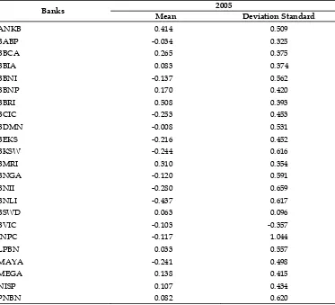
The next is on Table 2. This table reports the descriptive statistics of the logarithm of monthly equity returns and volatility banks of the sample
Table 2
Descriptive Statistics from Return Logarithms and Monthly Equity Volatility (2000-2005)
with DSb 12 and Volatility Asset (σV).
2005 Banks
Mean Deviation Standard
ANKB 0.414 0.509
BABP -0.034 0.325
BBCA 0.265 0.375
BBIA 0.083 0.374
BBNI -0.137 0.562
BBNP 0.170 0.420
BBRI 0.508 0.393
BCIC -0.253 0.453
BDMN -0.008 0.531
BEKS -0.216 0.452
BKSW -0.244 0.616
BMRI 0.310 0.354
BNGA -0.120 0.591
BNII -0.280 0.659
BNLI -0.437 0.617
BSWD 0.063 0.096
BVIC -0.103 -0.357
INPC -0.117 1.044
LPBN 0.033 0.557
MAYA -0.241 0.498
MEGA 0.138 0.415
NISP 0.107 0.434
for the period January 2000 - December 2005. All data were estimated using monthly basis by multi-plying the mean annual used with 12 and a stan-dard deviation with 12. The standard deviation of this will be an important input for the model prob-ability fail as inputs for determining the asset vola-tility (σV).
Table 2 shows the descriptive statistics of the logarithmic returns and volatility monthly equity of banks that were sampled for the period January 2000 to December 2005. All the data is estimated to be made monthly and yearly basis by multiplying the mean with 12 and standard deviation with. Standard deviation of the data will then be input to obtain the volatility of assets (σV).
When the volatility of the equity value is found, the next is to find the value of other inputs such as the market value of equity, debt value, and point failed. The failed point is assumed to be half of the total long-term debt plus all short-term debts. Time horizon (T) that is used is one-year time hori-zon. This time horizon is from the time of the audit which shows the time to the next audit performed within one year. Therefore, it is assumed that a
bank can survive in a period that has been targeted that within a year, even if the bank's assets cannot cover the total debt.
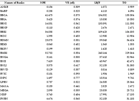
Since the calculation of risk-neutral probability of failed to require the presence of the risk free, this study uses the SBI as risk free. SBI is the average SBI 30 days, with an average value of 0.115 to 2005. As presented in Table 3, it shows the inputs for the calculation of risk neutral EDF. The market value of equity refers to the stock market data December 2005. For the debt and the data point fails (default point) refers to the financial statements as of 31 December 2005.
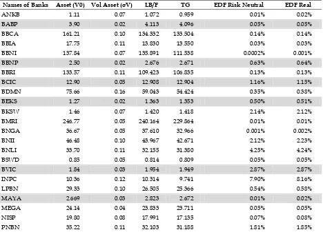
When such two non-linear equations of the model of Merton are done through numerical measures, the market value of assets and the vola-tility of asset values can be found. After that, the EDF risk neutral value is found easily. Table 4 below reports the market value of assets, asset volatility and EDF risk neutral.
Based on Table 4, there are some banks that the value of its assets falling below the failed point. They are Bank Bumiputra Indonesia, Bank Nusan-tara Parahyangan (BBNP), Bank Century (BCIC),
Table 3
The NPE, VE, LB or F, TG Referring to Capital Market 31 December 2005
Names of Banks NPE VE (σE) LB/F TG
ANKB 0.156 0.509 1.072 0.959
BABP 0.238 0.325 4.113 4.096
BBCA 41.473 0.375 134.332 133.504
BBIA 5.423 0.374 13.830 13.550
BBNI 16.831 0.562 135.891 111.538
BBNP 0.110 0.420 2.676 2.671
BBRI 36.038 0.393 109.423 106.835
BCIC 1.395 0.453 12.908 12.904
BDMN 23.075 0.531 59.043 54.424
BEKS 0.060 0.452 1.363 1.353
BKSW 0.199 0.500 1.420 1.418
BMRI 32.702 0.354 240.164 229.864
BNGA 3.161 0.508 37.610 32.966
BNII 7.419 0.585 43.967 42.671
BNLI 5.575 0.617 32.155 31.380
BSWD 0.129 0.337 0.814 0.809
BVIC 0.101 0.593 1.954 1.949
INPC 1.497 0.777 10.314 9.741
LPBN 5.737 0.522 26.505 25.366
MAYA 0.153 0.441 2.823 2.672
MEGA 2.893 0.335 23.833 23.711
NISP 3.763 0.434 17.991 17.135
the International Executive bank (BEKS), Bank Vic-toria International (BVIC), and the International Mayapada Bank (MAYA). The fall of the value of bank assets under point failed shows the condition of the bank's assets in 2005. This condition is indi-cated by the early warning Merton models for banks mentioned above.
Next is to separate the non-failed banks from failure in Indonesia. The bankruptcy law has not been implemented fully so as to make the bank as a bank fails normally that would impact the psycho-logical to the other banks in the banking system. Therefore, the way to determine when the bank has failed is consistent with the model of Merton such as when the failed point (default point) occurs is more prevalent in the period when the asset is equal to the number of short-term debt plus long-term debt 50%, hence the point fails then compared to the probability of failing.
It appears that this model can predict the bank failure well because the future of Bank Century operation permit is revoked by Bank Indonesia, failing to bailout. Bank Century license revocation by BI is considered a considerable burden by the
government or President Susilo Bambang Yud-hoyono (SBY). The failure concerns risk neutral
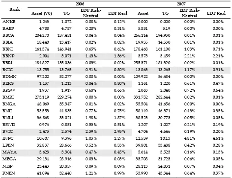
probability (EDF risk-neutral) and the Expected Default Frequency real (real EDF). The EDF value is the value of rating or the probability of failure can be used as input for the credit risk models. For test-ing the accuracy of the model, the Merton model, comparison is done that is between the probability of failure (Default Probability) banks that failed and did not fail to 2006 and 2007 with the results as presented in Table 5.
It appears that in 2006, only Bank Bumi Putra Indonesia (BABP) that could come out of the fall in the value of assets under point failed, while Bank Nusantara Parahyangan (BNBP), bank Cen-tury (BCIC), the Bank International Executive (BEKS), Bank Victoria International (BVIC), and the Bank International Mayapada (MAYA) are banks with assets still fall below the point failure (TG) as in 2005. In 2007, only Bank Century (BCIC) the value of its assets falls below the value of the point of failure (TG). This shows that the model of Merton can be a good predictor for probabilities of failure.
Table 4
The EDF Risk Neutral Value Showing V0 and σV Using Merton Model
Names of Banks Asset (V0) Vol Asset (σV) LB/F TG EDF Risk Neutral EDF Real
ANKB 1.11 0.07 1.072 0.959 0.01% 0.02%
BABP 3.90 0.02 4.113 4.096 0.05% 0.05%
BBCA 161.21 0.10 134.332 133.504 0.14% 0.14%
BBIA 17.75 0.11 13.830 13.550 0.03% 0.03%
BBNI 137.84 0.07 135.891 111.538 0.0002% 0.001%
BBNP 2.50 0.02 2.676 2.671 0.63% 0.64%
BBRI 133.57 0.11 109.423 106.835 0.13% 0.13%
BCIC 12.90 0.05 12.908 12.904 1.16% 1.15%
BDMN 75.66 0.16 59.043 54.424 0.35% 0.38%
BEKS 1.27 0.02 1.363 1.353 0.50% 0.51%
BKSW 1.46 0.07 1.420 1.418 2.14% 2.12%
BMRI 246.77 0.05 240.164 229.864 0.01% 0.01%
BNGA 36.67 0.05 37.610 32.966 0.001% 0.002%
BNII 46.48 0.10 43.967 42.671 2.12% 2.23%
BNLI 33.70 0.11 32.155 31.380 4.25% 4.24%
BSWD 0.85 0.05 0.814 0.809 0.05% 0.05%
BVIC 1.84 0.03 1.954 1.949 2.87% 2.87%
INPC 10.36 0.12 10.314 9.741 7.90% 8.16%
LPBN 29.33 0.10 26.505 25.366 0.54% 0.58%
MAYA 2.669 0.03 2.823 2.672 0.01% 0.02%
MEGA 24.14 0.04 23.833 23.711 0.05% 0.05%
NISP 19.80 0.08 17.991 17.135 0.07% 0.08%
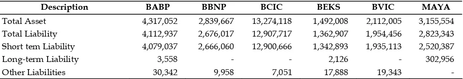
In finishing this research, it should still need further analysis. It shows that the position of the assets and liabilities of the six banks that have asset value (Vo) below the point of failure (TG) are such
as Bank Bumiputra Indonesia (BABP), Bank Nusan-tara Parhyangan (BBNP), Bank Century (BCIC), the Eksekutif Internasional (BEKS), bank Victoria In-ternational (BVIC) and the Bank Mayapada Inter-nasional (MAYA).
From Table 6, it appears that the three banks are Bank Nusantara Parahyangan (BBNP), Bank Century (BCIC ), and bank Victoria International (BVIC) has no long-term debt and most of the debt is short-term debt and other debt, and bank Cen-tury bank showed the highest risk to the amount of assets and liabilities are much larger than the other two banks.
Again, the data of banks’ assets and liabilities that have asset value (V0) is under the failure point
(TG). From the data bank's assets and liabilities is evident that Banks such as Bank Nusantara Para-hyangan (BNBP), Bank Century (BCIC), and Bank Victoria Internasional (BVIC) are the banks that do
not have long-term liabilities. They have almost all obligations that are short-term liabilities. These banks seem that the bank Century (BCIC) is a bank that has the highest risk because they are the largest banks in terms of assets and liabilities (more than four-time fold) compared to other risky banks. Assets and liabilities are based on data taken from the financial statements of Bank Century that is evident being lack of support for Merton models as predictors of bank failures models in terms of the support of the financial statements.
5. CONCLUSION, IMPLICATION, SUGGES-TION, AND LIMITATION
Now that this study concerns the application of BSM approach to predict the probability of the pub-lic banks that failed in Indonesia. It can be con-cluded that the model can predict the status of bankruptcy options with accurate even before the information given to the public. It is evidently the revocation of operating licenses of Bank Century later was identified and noted as the bank bailed
Table 5
(V0), (TG), EDF and EDF Real rRsk Neutral for 2006 and 2007
2006 2007 Bank
Asset (V0) TG EDF
Risk-Neutral EDF Real Asset TG
EDF
Risk-Neutral EDF Real
ANKB 1.243 1.072 0.08% 0.12% 0.000 0.000 0.00% 0.00%
BABP 4.788 4.787 0.28% 0.31% 5.851 5.19 0.00% 0.00%
BBCA 204.270 157.451 0.04% 0.04% 266.114 194.930 0.01% 0.01% BBIA 18.440 13.417 0.02% 0.02% 19.955 14.530 0.01% 0.01% BBNI 161.574 146.941 0.65% 0.62% 178.468 161.100 1.03% 0.71%
BBNP 2.904 3.071 1.43% 1.36% 3.573 3.459 2.21% 2.21%
BBRI 184.827 135.036 0.03% 0.02% 255.371 181.320 0.02% 0.01% BCIC 13.755 13.765 0.91% 0.80% 13.863 13.265 1.17% 0.91% BDMN 97.202 52.277 0.00% 0.00% 109.922 56.484 0.00% 0.00%
BEKS 1.137 1.213 0.84% 0.80% 1.161 1.220 0.61% 0.47%
BKSW 1.937 1.917 0.68% 0.66% 2.063 2.040 0.72% 0.64%
BMRI 273.119 229.274 0.00% 0.00% 331.752 282.644 0.02% 0.01% BNGA 48.069 35.347 0.01% 0.02% 55.504 41.656 0.00% 0.00% BNII 53.553 44.835 0.77% 0.75% 58.149 46.371 0.43% 0.35% BNLI 36.868 33.021 1.98% 1.87% 38.523 30.773 0.05% 0.05%
BSWD 0.974 0.851 0.53% 0.51% 1.207 1.027 0.21% 0.19%
BVIC 2.473 2.574 2.39% 2.95% 4.704 4.646 0.19% 0.20%
INPC 10.607 9.396 1.03% 1.27% 12.559 10.13 4.81% 4.61%
LPBN 32.837 28.666 0.52% 0.53% 39.801 33.488 0.42% 0.28%
MAYA 3.628 3.304 0.47% 0.45% 5.614 3.523 0.16% 0.13%
out by the government.
Furthermore, the model here not only provides an ordinal ranking of the banks used as the sample but also provide early warning of good predictabil-ity for the public. Besides that, this study is in line with research conducted by Bandyopadhyay (2007). Estimates based on the probability that the option may be an innovative approach to measure and manage credit risk in the future.
However, it has limitations and therefore sug-gestion must be asserted here. For example, for future research, it requires calibrating the probabil-ity of default (EDF Real) with a existing rater. By doing so, it can better get the rating that can be ap-proached rating for the institutions that have ex-isted.
REFERENCES
Altman, E 1968, ‘Financial ratios, discriminant analysis and the prediction of corporate bank-ruptcy’, Journal of Finance, Vol. 23, pp. 589-609. Altman, EI and Narayanan, P 1997, ‘Business
fail-ure classification models: an international sur-vey’, in Choi, FDS, Ed., International Accounting and Finance Handbook, John Wiley & Sons, New York, NY.
Arora, N, Bohn, JR and Zhu, F 2005, ‘Reduced form vs. structural models of credit risk: a case study of three models’, Journal of Investment Management, Vol. 3 No. 4, pp. 43-67.
Ayomi, S and Hermanto B 2013, ‘Systemic Risk and Financial Linkages Measurement in The Indo-nesian Banking’, Bulletin of Monetary, Economic and Banking.
Bandyopadhyay A 2007, ‘Mapping corporate drift towards default Part 1: a market-based ap-proach’, The Journal of Risk Finance, Vol. 8 No. 1, pp. 35-45
Black, F and Cox, JC 1976, ‘Valuing corporate secu-rities: some effects of bond indenture provi-sions’, Journal of Finance, Vol. 31 No. 2, pp. 351-67.
Black, F and Scholes, M 1973, ‘The pricing of op-tions and corporate liabilities’, Journal of
Politi-cal Economy, Vol. 81 No. 3, pp. 637-44.
Chen, RR, Chidambaran, NK, Immerman BM, So-prazentti JB 2012, Anatomy of Financial Institu-tion in Crisis : Endogenous Modeling of Bank
De-fault Risk, Fordham Graduate Scholl of
Busi-ness.
Davydenko, SA 2005, When do firms default? A study
of the default boundary, Mimeo, London
Busi-ness School.
Delianedis, R and Geske, R 2003, ‘Credit risk and risk neutral probabilities: information about rating migrations and defaults’, UCLA working
paper, University of California, Los Angeles,
CA.
Duffie, D and Singleton, K 1999, ‘Modeling the term structure of defaultable bonds’, Review of Financial Studies, Vol. 12 No. 4, pp. 687-720, JRF 8, 144.
Hadad, DM, Santoso, W, Besar, SD and Rulina, I 2004, ‘Probabilitas Kegagalan Korporasi Den-gan Menggunakan Model Merton’, Research paper, Biro Stabilitas Sistem Keuangan Direk-torat Penenlitian dan Pengaturan Perbankan Hull, JC 2002, Options, Futures, and Other
Deriva-tives, 5th ed, Prentice-Hall College Div, Saddle
River, NJ.
Kealhofer, S 2003, ‘Quantifying credit risk I: default prediction’, Financial Analysts Journal, Vol. 59 No. 1, pp. 30-44.
Kealhofer, S, Kwok, S and Weng, W 1998, ‘Uses and abuses of bond default rates’, Working paper, KMV Corporation, San Francisco, CA.
Kulkarni A, Mishra AK and Thakker J 2012, How Goods is Merton Model at Assessing Credit Risk
Evidence from India, National Institute of Bank
Management
Leland, HE 1994, ‘Corporate debt value, bond covenants, and the optimal capital structure’,
Journal of Finance, Vol. 49 No. 4, pp. 1213-52. Leland, HE 2002, ‘Predictions of expected default
frequencies in structural models of debt’, Work-ing paper, University of California, Los Angeles, CA.
Merton, RC 1974, ‘On the pricing of corporate debt:
Table 6
List of Assets and Liabilities in Millions of Rupiah Banks Has Asset Value (Vo) < the point of failure (TG) and Debt 2005
Description BABP BBNP BCIC BEKS BVIC MAYA
Total Asset 4,317,052 2,839,667 13,274,118 1,492,008 2,112,005 3,155,554 Total Liability 4,112,937 2,676,017 12,907,717 1,362,907 1,954,456 2,823,343 Short tem Liability 4,079,037 2,666,060 12,900,666 1,342,893 1,935,113 2,520,387
Long-term Liability 3,558 - - 2,126 - 302,956
The risk structure of interest rates’, Journal of Finance, Vol. 29 No. 2, pp. 449-70.
Moody’s, KMV 2003, ‘Modeling default risk’,
Tech-nical working paper, 18 December, Moody’s
KMV, San Francisco, CA.
Vasicek, OA, 1984, ‘Credit valuation’, Unpublished
paper, KMV Corporation, San Francisco, CA.