DOI: 10.12928/TELKOMNIKA.v13i2.1322 547
Experimental Validation of a Multi Model PI Controller
for a Non Linear Hybrid System in LabVIEW
M.Kalyan Chakravarthi*1,Nithya Venkatesan2 School of Electronics Engineering,
VIT University, Vandalur-Kelambakkam road, Chennai, Tamil Nadu, India 600127 *Corresponding author, e-mail: [email protected], [email protected]
Abstract
In this paper a real time Single Spherical Tank Liquid Level System (SSTLLS) has been chosen for investigation. This paper describes the design and development of a Multi Model PI Controller (MMPIC) using classical controller tuning techniques for a single spherical nonlinear tank system. System identification of these different regions of nonlinear process are done using black box modeling, which is identified to be nonlinear and approximated to be a First Order Plus Dead Time (FOPDT) model. A proportional and integral controller is designed using LabVIEW and Chen-Hrones-Reswick (CHR), Zhuang-Atherton (ZA), and Skogestad’s Internal Model Controller (SIMC) tuning methods are implemented in real time. The paper provides the details about the data acquisition unit, shows the implementation of the controller and comparision of the results of PI tuning methods used for an MMPI Controller.
Keywords: Graphical User Interface (GUI), PI Controller, Chen-Hrones-Reswick (CHR), Zhuang-Atherton (ZA), and Skogestad’s Internal Model Controller (SIMC), LabVIEW
1. Introduction
In common terms, most of the industries have typical problems raised because of the dynamic non linear behavior of the storage tanks. It’s only because of the inherent non linearity, most of the chemical process industries are in need of classical control techniques. Hydrometallurgical industries, food process industries, concrete mixing industries and waste water treatment industries have been actively using the spherical tanks as an integral process element. Due to its changing cross section and non linearity, a spherical tank provides a challenging problem for the level control.
SSTLLS has been a model for quite a many experiments performed in the near past. Nithya et al [7] have designed a model based controller for a spherical tank, which gave a comparison between IMC and PI controller using MATLAB. Naresh Nandola et al [8] have studied and mathematically designed a predictive controller for non linear hybrid system. A gain scheduled PI controller was designed using a simulation on MATLAB for a second order non linear system by Dinesh Kumar et al [9] which gave information about servo tracking for different set points. A fractional order PID controller was designed for liquid level in spherical tank using MATLAB, which compared the performance of fractional order PID with classical PI controller by Sundaravadivu et al [10]. Kalyan Chakravarthi et al have implemented a classical and gain scheduled PI controllers for a single and dual spherical tank systems in real time using LabVIEW [11],[12]. An adaptive fuzzy PID controller has been implemented for controlling level process [13]. A Fuzzy Immune PID Control was also implemented on a hydraulic system ,which was optimized by PSO algorithm [14].
2. Experimental Process Description
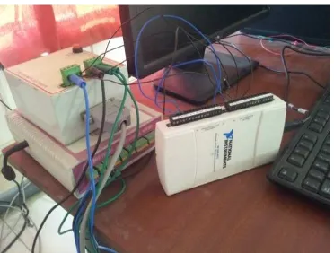
The laboratory set up for this system basically consists of two spherical interacting tanks which are connected with a manually operable valve between them. Both the tanks have an inflow and outflow of water which is being pumped by the motor, which continuously feeds in the water from the water reservoir. The flow is regulated in to the tanks through the pneumatic control valves, whose position can be controlled by applying air to them.
Figure 1. Real time experimental set up of the process
Figure 2. Interfaced NI-DAQmx 6211 Data Acquisition Module Card
the signal provided by I/P converter which in turn regulates the flow of water in to the tank. Figure 2 shows the interfaced NI-DAQmx 6211 data acquisition card.
3. System Identification and Controller Design 3.1. Mathematical Modeling of SSTLLS
The SSTLLS is a system which is non linear in nature by virtue of its varying diameter. The dynamics of this non linearity can be described by the first order differential equation.
= q1 - q2 (1)
Where, V is the volume of the tank, q1 is the Inlet flow rate and, q2 is the Outlet flow rate. The
volume V of the spherical tank is given by,
V= h3 (2)
Where h is the height of the tank in cm.
On application of the steady state values, and by solving the equations 1 and 2, the non linear spherical tank can be linearized to the following model,
(3)
Where, τ = 4πRt hS and
The system identification of SSTLLS is derived using the black box modeling. Under constant inflow and constant outflow rates of water, the tank is allowed to fill from (0-45) cm. Each sample is acquired by NI-DAQmx 6211 from the differential pressure transmitter through USB port in the range of (4-20) mA and the data is transferred to the PC.This data is further scaled in terms of level in cm.Employing the open loop method, for a given change in the input variable; the output response of the system is recorded. Ziegler and Nichols [5] have obtained the time constant and time delay of a FOPDT model by constructing a tangent to the experimental open loop step response at its point of inflection. The intersection of the tangent with the time axis provides the estimate of time delay. The time constant is estimated by calculating the tangent intersection with the steady state output value divided by the model gain. Cheng and Hung [15] have also proposed tangent and point of inflection methods for estimating FOPDT model parameters. The major disadvantage of all these methods is the difficulty in locating the point of inflection in practice and may not be accurate. Prabhu and Chidambaram [16] have obtained the parameters of the first order plus time delay model from the reaction curve obtained by solving the nonlinear differential equations model of a distillation column. Sundaresan and Krishnaswamy [17] have obtained the parameters of FOPDT transfer function model by collecting the open loop input-output response of the process and that of the model to meet at two points which describe the two parameters τp and θ. The proposed times t1 and t2,
are estimated from a step response curve. The proposed times t1 and t2, are estimated from a
step response curve. This time corresponds to the 35.3% and 85.3% response times. The time constant and time delay are calculated as follows.
τp = 0.67(t2− t1) (4)
θ = 1.3t1− 0.29t2 (5)
plant. The S-shaped curve may be characterized by two constants, delay time L and time constant τ. The experimental data are approximated to be an FOPDT model.
3.2. Design of PI Controller
The derivation of transfer function model will now pave the way to the controller design which shall be used to maintain the system to the optimal set point. This can be only obtained by properly selecting the tuning parameters Kp and Ki for a PI controller.
The conventional FOPDT model is given by,
G(s) = (7)
Table 1 gives the transfer functions designed for different regions of SSTLLS. It can be noticed that the delay exponentially increases as the degree of non linearity increases. The transfer function models are derived for five different regions across the varying diameter of SSTLLS.
By implementing the rules of PI tuning by the methods ZA, CHR and SIMC methods to get the following parameters for the transfer function specified in Table 1.The parameters of Kp
and Ki for different regions of non linearity are derived and given in Table 2.
Table 1. Transfer function models for different regions of SSTLLS
Region of Operation Transfer Function
0-9
9-18
18-27
27-36
36-45
4. Results and Discussions
The CHR, ZA and SIMC based MMPI controllers which were designed and are implemented using the graphical programming code which is written on LabVIEW. These controllers were applied to SSTLLS and the performance of them was compared under different condition and regions of operation.
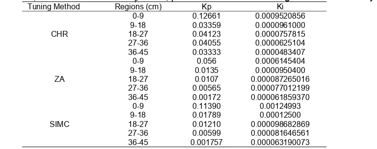
Table 2. CHR, ZA and SIMC tuned Kp and Ki parameters for different regions of non linearity
Tuning Method Regions (cm) Kp Ki
CHR
0-9 0.12661 0.0009520856
9-18 0.03359 0.0000961000
18-27 0.04123 0.0000757815
27-36 0.04055 0.0000625104
36-45 0.03333 0.0000483407
ZA
0-9 0.056 0.0006145404
9-18 0.0135 0.0000950400
18-27 0.0107 0.000087265016
27-36 0.00565 0.000077012199
36-45 0.00172 0.000061859370
SIMC
0-9 0.11390 0.00124993
9-18 0.01789 0.00012500
18-27 0.01210 0.000098682869
27-36 0.00599 0.000081646561
4.1. Changes in the Load
The CHR, ZA and SIMC tuned controllers have been used to control the level of SSTLLS while applying a load change of 7.5% for a set of set points. Initially to test the response of the tank in its non linear region, a set point of 4.5 cm was fed to the program and the readings were recorded. Similar method was employed for the set points of 2.25, and 9 cm respectively. While applying a set point of 2.25 from 4.5 cm, we are intending to observe the negative set point tracking performance.
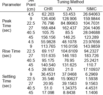
Table 3. Comparison of Time Domain Analysis for Servo Response for different regions
Parameter
4.5 62.203 53.453 26.64063
9 126.406 128.906 159.9844
22.5 76.796 84.89063 104.7031 27 168.484 162.437 204.1406
40.5 105.75 85.5 28.04688
45 156.156 146.25 123.289
Rise Time (sec)
4.5 55.9828 48.1078 23.97656
9 113.765 116.0156 143.9859
22.5 69.117 104.6109 94.2327 27 151.635 146.193 183.726 40.5 95.175 76.95 25.2421 45 140.540 131.625 110.7
Settling Time (sec)
4.5 28.953 21.0 17.10937
9 36.4531 37.0468 6.2969
22.5 35.546 15.90627 1.5938 27 20.95 39.1563 9.1563 40.5 51.0 1.34375 4.4531 45 17.098 8.8438 1.1406
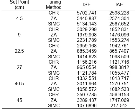
The similar process of observing the negative set point tracking is also adopted. At all the levels, a disturbance is added to the system to observe its performance. Similarly the set points are changed for the regions of 18-27 cm and 36-45 cm in the SSTLLS. Figures 3(a), 3(b), 3(c), 3(d), 3(e), 3(f), 3(g), 3(h), 3(i) demonstrate the regulatory performance under the influence of external disturbance of tuned MMPI controller in the regions of 0-9 cm, 18-27 cm and 36-45 cm for CHR, ZA and SIMC tuned MMPI controllers respectively. The performance indices of the regulatory response can be seen in Table 5.The designed controllers were able to compensate the effect of the load changes.It can be noticed from Table 5, that the ISE and IAE values for SIMC method are relatively lesser than the ZA and CHR method in the regions 0-9 cm and 36-45 cm of SSTLLS, where the degree of non linearity is very high.At the same time it can be seen that, in all the other regions of operation ZA tuned MMPI controller shows an efficient disturbance rejection and provides relatively lesser ISE and IAE values across the regions 9-18 cm, 18-27 cm, 27-36 cm.
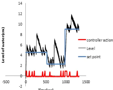
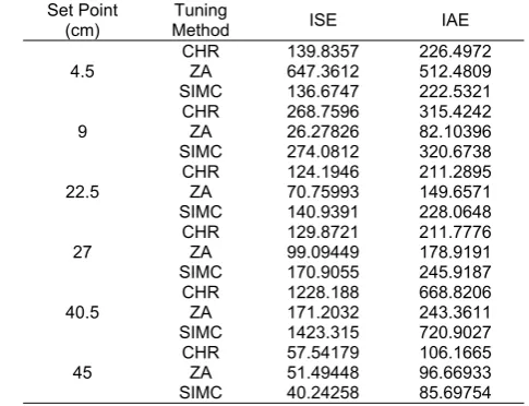
4.2. Variation of the Set Point
SIMC method in non linear region of 4.5cm and 40cm are less when compared to that CHR and ZA method. If keenly observed, SIMC tuned controller performs better than that of other two methods with respect to ISE and IAE calculations. It can be inferred that for faster time response in non linear regions SIMC method of tuning proves to be the best method. But if the emphasize is more on the error reduction in the system, ZA method gives a best of its performance in almost all the regions of operations. It can be very well seen that extreme non linear regions 0-9cm and 36-45cm have a very less IAE and ISE, thus proving the efficiency of SIMC tuning method over the ZA and CHR method.
Figure 3(a). ZA tuned MMPI Controller’s Regulatory Response for region 0-9cm
Figure 3(b). SIMC tuned MMPI Controller’s Regulatory Response for region 0-9cm
Figure 3(c).CHR tuned MMPI Controller’s Regulatory Response for region 0-9cm
Figure 3(e). SIMC tuned MMPI Controller’s Regulatory Response for region 18-27cm
Figure 3(f). CHR tuned MMPI controller’s Regulatory Response for region 18-27cm
Figure 3(g). ZA tuned MMPI Controller’s Regulatory Response for region 36-45cm
Figure 3(h). SIMC tuned MMPI Controller’s Regulatory Response for region 36-45cm
Table 4. Comparison of performance indices of servo response for different regions
Set Point (cm)
Tuning
Method ISE IAE
4.5
CHR 139.8357 226.4972
ZA 647.3612 512.4809
SIMC 136.6747 222.5321
9
CHR 268.7596 315.4242
ZA 26.27826 82.10396
SIMC 274.0812 320.6738
22.5
CHR 124.1946 211.2895
ZA 70.75993 149.6571
SIMC 140.9391 228.0648
27
CHR 129.8721 211.7776
ZA 99.09449 178.9191
SIMC 170.9055 245.9187
40.5
CHR 1228.188 668.8206
ZA 171.2032 243.3611
SIMC 1423.315 720.9027
45
CHR 57.54179 106.1665
ZA 51.49448 96.66933
Figure 3(i). CHR tuned MMPI controller’s Regulatory Response for region 36-45cm
Figure 4(a).Servo Responses of CHR, ZA and SIMC tuned MMPI controllers for region 0-9cm
Figure 4(b). Servo Responses of CHR,ZA and SIMC tuned MMPI controllers for region
18-27cm
Figure 4(c).Servo Responses of CHR, ZA and SIMC tuned MMPI controllers for region
36-45cm
Table 5. Comparison of performance Indices of regulatory response in different regions
Set Point (cm)
Tuning
Method ISE IAE
4.5
CHR 5702.741 2598.228
ZA 5440.887 2574.304
SIMC 5134.143 2567.652
9
CHR 3029.299 1852.831
ZA 1979.908 1476.096
SIMC 2231.789 1553.274
22.5
CHR 2959.168 1942.761
ZA 885.3459 865.7407
SIMC 1414.623 1098.509
27
CHR 1156.216 1121.716
ZA 965.0554 998.3812
SIMC 1121.784 1055.477
40.5
CHR 1332.551 1013.717
ZA 3011.964 1270.751
SIMC 1056.572 1082.533
45
CHR 250.7785 456.9153
ZA 3289.437 1747.069
SIMC 107.6896 217.542
4. Conclusion
NI-DAQmx 6211 data acquisition card and LabVIEW. Graphical programming was used to implement the whole experiment. The experimental results evidently prove that the influence of set point and load changes are smooth for SIMC method of tuning in non linear regions. It can be also seen that minimum overshoot, faster settling time and rise time are obtained. It has a better capability of compensating all the load changes. In the regions of lesser degree of non linearity ZA method proves to be relatively effective for it provides smaller values of ISE,IAE and all the time indices. The ISE and IAE values justify that relatively a minimum error is seen in SIMC way of tuning the MMPI PI controller than ZA and CHR methods for both servo and regulatory responses..It can be concluded that SIMC method based MMPI PI controller can be implemented in extreme non linear regions on real time SSTLLS using NI-DAQmx 6211 data acquisition module and LabVIEW in real time.
References
[1] Biegler LT, Rawlings JB. Optimization approaches to nonlinear model predictive control. In chemical process control, CPCIV. 1991: 543-571.
[2] Kravaris C, Arkun Y. Geometric nonlinear control-An Overview International journal of chemical process control, CPCIV. 1991: 477-515.
[3] Raich A, Wu X, Cinar A. A comparative study of neural networks and nonlinear time series modeling techniques. AIChE Conference. Los Angeles, CA. 1991.
[4] George KI, Boa GH, Raymand. Analysis of direct action fuzzy PID controller structures. IEEE Trans.on SMC. 1999; 29(3): 371-388.
[5] Ziegler JG, Nicolas NB. Optimum settings for automatic controllers. Transactions of ASME. 1942; 64: 759-768.
[6] Zhuang M, Atherton DP. Automatic tuning of optimum PID controllers. Proceedings of IEEE. 1993; 140(3): 216-224.
[7] S Nithya, N Sivakumaran, T Balasubramanian, N Anantharaman. Modelbased controller design for a spherical tank process in real time. IJSSST. 2008; 9(4).
[8] Naresh NN, Sharad B. A multiple model approach for predictive control of nonlinear hybrid systems. Journal of process control. 2008; 18: 131-148.
[9] D Dinesh K, B Meenakshipriya. Design and implementation of non linear system using gain scheduled PI controller. Procedia engineering. 2012; 38: 3105-3112.
[10] K Sundaravadivu, K Saravanan. Design of fractional order PID Controller for liquid level control of spherical tank. European journal of Scientific Research. 2012; 84(3): 345-353.
[11] M Kalyan C, Nithya V. LabVIEW Based Tuning Of PI Controllers For A Real Time Non Linear Process. Journal of Theoretical and Applied Information Technology. 2014; 3(5): 579-585.
[12] M Kalyan C, Pannem KV, Nithya V. Real Time Implementation of Gain Scheduled Controller Design for Higher Order Nonlinear System Using LabVIEW. International Journal of Engineering and Technology. 2014; 6(5): 2031-2038.
[13] Ke Z, Jingxian Q, Jia S, Shizhong C, Yuhou W. Application of Adaptive Fuzzy PID Leveling Controller. TELKOMNIKA Indonesian Journal of Electrical Engineering. 2013; 11(5): 2869-2878. [14] Ma Y, Gu L. Fuzzy Immune PID Control of Hydraulic System based on PSO Algorithm.
TELKOMNIKA Indonesian Journal of Electrical Engineering. 2013; 11(2): 890-895.
[15] GS Cheng, JC Hung. A least-square based self tuning of PID Controller. Proc. IEEE South East Conference, North Carolina. 1985: 325-332.
[16] ES Prabhu, M Chidambaram. Robust control of a distillation coloumn by method of inequalities. Indian Chen.Engr. 1991; 37: 181-187.