ESTIMATING ABOVE GROUND TREES BIOMASS
OF FOREST COVER USING
FIELD MEASUREMENT AND QUICKBIRD IMAGE
IN LORE LINDU NATIONAL PARK-CENTRAL SULAWESI
NAIMATU SOLICHA
GRADUATE SCHOOL
STATEMENT
I, Naimatu Solicha, here by stated that this thesis entitled:
Estimating Above Ground Trees Biomass of Forest Cover Using Field Measurement and Quickbird Image In Lore Lindu National Park-Central Sulawesi
are results of my work during the period of June February until August 2007 and it has not been published before. The content of the thesis has been examined by the advising committee and the external examiner.
Bogor, August 2007
ACKNOWLEDGMENT
This thesis was completed with the support of STORMA program. STORMA stands for Stability of Rainforest Margin in Indonesia is an Indonesian-German collaboration research funded by the Indonesian-German Research Foundation (FDG). I would like to give my highly appreciation to FDG-STORMA for the research support and the following people that give a high encouragement and help to finish my thesis:
1. My family for giving the unwavering faith and support me to finish my master degree.
2. Dr. Tania June, Dr. Antonius B.W. and Dr. M. Ardiansyah as my supervisor and co-supervisors for their guidance, help, idea, comment and constructive criticism during my research.
3. Dr. M. Buce Saleh as the external examiner for his positive inputs and ideas.
4. Dr. Surya Tarigan, Dr. Adam Malik and Mr. Wolfram Lorenz as the STORMA coordinators of IPB, Untad and German for their assistance during the implementation of research.
5. Mr. Abdul Rauf and Mr. Heiner as STORMA B1 Sub Program Coordinator for helping to arrange the field observation, discussion and their positive input and idea.
6. My friend in MIT IPB for helping and supporting me in finishing thesis and pass our ups and down during finishing our master degree.
7. Kak Amran and all of STORMA assistants for giving kindness, help, assistance, support me during the field observation in Sulawesi.
8. Adhi Tyan Wijaya for moral support, positive suggestion and his patience accompany and listen to my problems in finishing my master degree. 9. MIT secretariat and all staff for helping me to arrange the administration,
technical and facilities.
CURRICULUM VITAE
Naimatu Solicha was born in Surabaya, East Java Indonesia on October 1st 1982. She was graduated from Brawijaya University, Agricultural Faculty, and Agronomy Department in 2004. She was entered the IPB Graduate School in year 2005. Before entering the Graduate School of Bogor Agricultural University she worked as assistant lecturer in Brawijaya University and as private English tutor.
ABSTRACT
NAIMATU SOLICHA (2007). “Estimating above ground trees biomass of forest cover using field measurement and QuickBird image in Lore Lindu National Park-Central Sulawesi” under supervision of Dr. Tania June, Dr. Antonius B.W and Dr. M. Ardiansyah
Forests play an important role in global carbon cycling, since they hold a large pool of carbon as well as potential carbon sinks and sources to the atmosphere. Accurate estimation of forest biomass is required for greenhouse gas inventories and terrestrial carbon accounting (Muukkonen and Heiskanen, 2006). The biomass of forest provides estimates of the carbon pools in forest vegetation because about 50% of it is carbon. Direct measurement of biomass on the ground is time consuming (expensive), and repeated measurements, if they occur at all, are generally limited to 10 year interval. The possibility that above ground forest biomass can be determined from space is a promising alternative to ground-based methods. Remote sensing has opened an effective way to estimate forest biomass and carbon. By the combination of data field measurement and allometric equation, the above ground trees biomass is possible to be estimated over the large area.
The objectives of this research are: (1) To estimate the above ground tree biomass and carbon stock of forest cover in Lore Lindu National Park by combination of field data observation, allometric equation and multispectral satellite image; (2) to find the equation model between parameter that determines the biomass estimation.
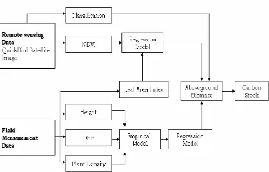
The method of this research use an approach of estimating the biomass that combines field studies (forest inventory data), analysis of multispectral satellite imagery, allometric equation and statistical analysis. Forest cover type classification was utilized for analyzing the biomass per pixel in each different cover type. The classifications for each cover type by using the region based different spectral value in each observation plot refer to QuickBird Image.
TABLE OF CONTENTS
STATEMENT ... ii
ACKNOWLEDGMENT... iii
CURRICULUM VITAE ... iv
ABSTRACT... v
TABLE OF CONTENTS... ii
LIST OF FIGURES ... ix
LIST OF TABLES ... xii
I. INTRODUCTION ... 1
1.1 Background ... 1
1.2 Objectives... 4
1.3 Output... 5
1.4 Thesis Outline ... 5
II. LITERATURE REVIEW... 7
2.1 Biomass and Carbon Stock ... 7
2.1.1 Definition of Biomass ... 7
2.1.2 Biomass Estimation... 8
2.1.3 Methods for Estimating Biomass Density from Existing Data... 9
2.1.4 Carbon Stock... 16
2.1.5 Carbon stock measurement ... 16
2.2 Remote Sensing... 18
2.2.1 Remote Sensing Application in Forestry ... 19
2.2.2 Remote Sensing for Aboveground Biomass Estimation... 21
2.2.3 Different Satellite Images in Biomass and C-Stock Estimation ... 22
2.2.4 Remote Sensing Estimation of LAI ... 23
2.2.5 Vegetation Indices... 24
2.3 Empirical Modeling ... 29
III. RESEARCH METHODOLOGY... 31
3.1 Time and Location ... 31
3.2 Data Source ... 32
3.2.1 Remote Sensing Data ... 33
3.2.2 Field Measurement Data ... 33
3.3 Method ... 33
3.4 Forest Cover Type Classification... 34
3.5 Vegetation Index ... 36
3.6 Field Data Measurement ... 36
3.7 Calculating Biomass using Allometric Equation (ton/ha) ... 38
3.8 Calculating Carbon-Stock (ton/ha) ... 39
3.9 Statistical Analysis ... 39
3.9.1 Standard deviation... 39
3.9.2 Correlation Coefficients ... 40
3.9.3 Correlation between the parameter ... 41
3.11 Research Schedule ... 43
IV. RESULT AND DISCUSSION ... 44
4.1 Field Data Measurement ... 44
4.2 Forest cover type classification using Quick Bird image... 49
4.3 Correlation between the parameters... 51
4.3.1 Biomass and Diameter Breast Height (DBH) ... 52
4.3.2 Biomass and Total Height... 59
4.3.3 Biomass and LAI ... 65
4.3.4 Biomass and NDVI ... 66
4.3.5 LAI and NDVI ... 66
4.4 Model analysis ... 67
4.4.1 Comparison between field and biomass model... 69
4.5 Biomass and Carbon Stock Estimation ... 72
4.5.1 Comparison between research result with other published data ... 74
V. CONCLUSION AND RECOMMENDATION ... 77
5.1 Conclusion ... 77
5.2 Recommendation ... 78
REFERENCE... 79
LIST OF FIGURES
Figure 3.1 Research Study Area. ... 32
No. Caption Page Figure 3.2 General procedure of biomass and carbon stock estimation. ... 34
Figure 3.3 Forest covers type classification procedure... 35
Figure 3.4 The sampling scheme for field measurement data. ... 37
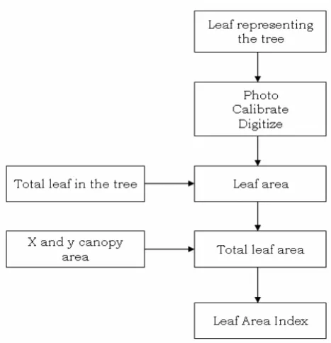
Figure 3.5 General flow of LAI field measurement... 38
Figure 4.1 Plot distribution of field data observation. ... 45
Figure 4.2 Plot observation for cover type A and B. ... 47
Figure 4.3 Plot observation for cover type C and D. ... 48
Figure 4.4 Image of STORMA project area and study area. ... 49
Figure 4.5 Forest covers type classification of Quick Bird image... 50
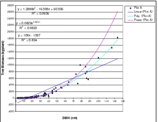
Figure 4.6 Tree biomass and DBH of forest cover type A using polynomial regression. ... 52
Figure 4.7 Tree biomass and DBH of forest cover type B using polynomial regression. ... 53
Figure 4.8 Tree biomass and DBH of forest cover type B using power regression. ... 54
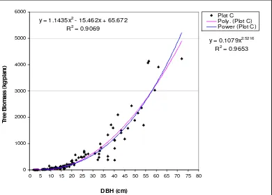
Figure 4.9 Tree biomass and DBH of forest cover type C using power regression. ... 54
Figure 4.10 Tree biomass and DBH of forest cover type D using polynomial regression. ... 55
Figure 4.11 Tree biomass and DBH of forest cover type D using power regression. ... 55
Figure 4.12 Tree biomass and DBH correlation regression model of forest cover type A ... 56
Figure 4.13 Tree biomass and DBH correlation regression model of forest cover type B. ... 57
Figure 4.15 Tree biomass and DBH correlation regression model of forest
cover type D. ... 58
Figure 4.16 Tree biomass and DBH correlation regression model of tropical rain forest covering type A, B, C and D... 58
Figure 4.17 Tree biomass and total height of forest cover type A using power regression. ... 60
Figure 4.18 Tree biomass and total height of forest cover type B using power regression. ... 60
Figure 4.19 Tree biomass and total height of forest cover type C using power regression. ... 61
Figure 4.20 Tree biomass and total height of forest cover type D using polynomial regression. ... 61
Figure 4.21 Tree biomass and total height correlation regression model of forest cover type A. ... 62
Figure 4.22 Tree biomass and total height correlation regression model of forest cover type B. ... 63
Figure 4.23 Tree biomass and total height correlation regression model of forest cover type C. ... 63
Figure 4.24 Tree biomass and total height correlation regression model of forest cover type D. ... 64
Figure 4.25 Tree biomass and DBH correlation regression model of tropical rain forest covering type A, B, C and D... 64
Figure 4.26 Trees biomass and LAI correlation... 65
Figure 4.27 Biomass and NDVI image correlation of each cover type. ... 66
Figure 4.28 LAI and NDVI image correlation... 67
Figure 4.29 DBH on field and model trees biomass comparison of forest cover type A. ... 69
Figure 4.30 DBH on field and model trees biomass comparison of forest cover type B. ... 69
ESTIMATING ABOVE GROUND TREES BIOMASS
OF FOREST COVER USING
FIELD MEASUREMENT AND QUICKBIRD IMAGE
IN LORE LINDU NATIONAL PARK-CENTRAL SULAWESI
NAIMATU SOLICHA
GRADUATE SCHOOL
STATEMENT
I, Naimatu Solicha, here by stated that this thesis entitled:
Estimating Above Ground Trees Biomass of Forest Cover Using Field Measurement and Quickbird Image In Lore Lindu National Park-Central Sulawesi
are results of my work during the period of June February until August 2007 and it has not been published before. The content of the thesis has been examined by the advising committee and the external examiner.
Bogor, August 2007
ACKNOWLEDGMENT
This thesis was completed with the support of STORMA program. STORMA stands for Stability of Rainforest Margin in Indonesia is an Indonesian-German collaboration research funded by the Indonesian-German Research Foundation (FDG). I would like to give my highly appreciation to FDG-STORMA for the research support and the following people that give a high encouragement and help to finish my thesis:
1. My family for giving the unwavering faith and support me to finish my master degree.
2. Dr. Tania June, Dr. Antonius B.W. and Dr. M. Ardiansyah as my supervisor and co-supervisors for their guidance, help, idea, comment and constructive criticism during my research.
3. Dr. M. Buce Saleh as the external examiner for his positive inputs and ideas.
4. Dr. Surya Tarigan, Dr. Adam Malik and Mr. Wolfram Lorenz as the STORMA coordinators of IPB, Untad and German for their assistance during the implementation of research.
5. Mr. Abdul Rauf and Mr. Heiner as STORMA B1 Sub Program Coordinator for helping to arrange the field observation, discussion and their positive input and idea.
6. My friend in MIT IPB for helping and supporting me in finishing thesis and pass our ups and down during finishing our master degree.
7. Kak Amran and all of STORMA assistants for giving kindness, help, assistance, support me during the field observation in Sulawesi.
8. Adhi Tyan Wijaya for moral support, positive suggestion and his patience accompany and listen to my problems in finishing my master degree. 9. MIT secretariat and all staff for helping me to arrange the administration,
technical and facilities.
CURRICULUM VITAE
Naimatu Solicha was born in Surabaya, East Java Indonesia on October 1st 1982. She was graduated from Brawijaya University, Agricultural Faculty, and Agronomy Department in 2004. She was entered the IPB Graduate School in year 2005. Before entering the Graduate School of Bogor Agricultural University she worked as assistant lecturer in Brawijaya University and as private English tutor.
ABSTRACT
NAIMATU SOLICHA (2007). “Estimating above ground trees biomass of forest cover using field measurement and QuickBird image in Lore Lindu National Park-Central Sulawesi” under supervision of Dr. Tania June, Dr. Antonius B.W and Dr. M. Ardiansyah
Forests play an important role in global carbon cycling, since they hold a large pool of carbon as well as potential carbon sinks and sources to the atmosphere. Accurate estimation of forest biomass is required for greenhouse gas inventories and terrestrial carbon accounting (Muukkonen and Heiskanen, 2006). The biomass of forest provides estimates of the carbon pools in forest vegetation because about 50% of it is carbon. Direct measurement of biomass on the ground is time consuming (expensive), and repeated measurements, if they occur at all, are generally limited to 10 year interval. The possibility that above ground forest biomass can be determined from space is a promising alternative to ground-based methods. Remote sensing has opened an effective way to estimate forest biomass and carbon. By the combination of data field measurement and allometric equation, the above ground trees biomass is possible to be estimated over the large area.
The objectives of this research are: (1) To estimate the above ground tree biomass and carbon stock of forest cover in Lore Lindu National Park by combination of field data observation, allometric equation and multispectral satellite image; (2) to find the equation model between parameter that determines the biomass estimation.
The method of this research use an approach of estimating the biomass that combines field studies (forest inventory data), analysis of multispectral satellite imagery, allometric equation and statistical analysis. Forest cover type classification was utilized for analyzing the biomass per pixel in each different cover type. The classifications for each cover type by using the region based different spectral value in each observation plot refer to QuickBird Image.
TABLE OF CONTENTS
STATEMENT ... ii
ACKNOWLEDGMENT... iii
CURRICULUM VITAE ... iv
ABSTRACT... v
TABLE OF CONTENTS... ii
LIST OF FIGURES ... ix
LIST OF TABLES ... xii
I. INTRODUCTION ... 1
1.1 Background ... 1
1.2 Objectives... 4
1.3 Output... 5
1.4 Thesis Outline ... 5
II. LITERATURE REVIEW... 7
2.1 Biomass and Carbon Stock ... 7
2.1.1 Definition of Biomass ... 7
2.1.2 Biomass Estimation... 8
2.1.3 Methods for Estimating Biomass Density from Existing Data... 9
2.1.4 Carbon Stock... 16
2.1.5 Carbon stock measurement ... 16
2.2 Remote Sensing... 18
2.2.1 Remote Sensing Application in Forestry ... 19
2.2.2 Remote Sensing for Aboveground Biomass Estimation... 21
2.2.3 Different Satellite Images in Biomass and C-Stock Estimation ... 22
2.2.4 Remote Sensing Estimation of LAI ... 23
2.2.5 Vegetation Indices... 24
2.3 Empirical Modeling ... 29
III. RESEARCH METHODOLOGY... 31
3.1 Time and Location ... 31
3.2 Data Source ... 32
3.2.1 Remote Sensing Data ... 33
3.2.2 Field Measurement Data ... 33
3.3 Method ... 33
3.4 Forest Cover Type Classification... 34
3.5 Vegetation Index ... 36
3.6 Field Data Measurement ... 36
3.7 Calculating Biomass using Allometric Equation (ton/ha) ... 38
3.8 Calculating Carbon-Stock (ton/ha) ... 39
3.9 Statistical Analysis ... 39
3.9.1 Standard deviation... 39
3.9.2 Correlation Coefficients ... 40
3.9.3 Correlation between the parameter ... 41
3.11 Research Schedule ... 43
IV. RESULT AND DISCUSSION ... 44
4.1 Field Data Measurement ... 44
4.2 Forest cover type classification using Quick Bird image... 49
4.3 Correlation between the parameters... 51
4.3.1 Biomass and Diameter Breast Height (DBH) ... 52
4.3.2 Biomass and Total Height... 59
4.3.3 Biomass and LAI ... 65
4.3.4 Biomass and NDVI ... 66
4.3.5 LAI and NDVI ... 66
4.4 Model analysis ... 67
4.4.1 Comparison between field and biomass model... 69
4.5 Biomass and Carbon Stock Estimation ... 72
4.5.1 Comparison between research result with other published data ... 74
V. CONCLUSION AND RECOMMENDATION ... 77
5.1 Conclusion ... 77
5.2 Recommendation ... 78
REFERENCE... 79
LIST OF FIGURES
Figure 3.1 Research Study Area. ... 32
No. Caption Page Figure 3.2 General procedure of biomass and carbon stock estimation. ... 34
Figure 3.3 Forest covers type classification procedure... 35
Figure 3.4 The sampling scheme for field measurement data. ... 37
Figure 3.5 General flow of LAI field measurement... 38
Figure 4.1 Plot distribution of field data observation. ... 45
Figure 4.2 Plot observation for cover type A and B. ... 47
Figure 4.3 Plot observation for cover type C and D. ... 48
Figure 4.4 Image of STORMA project area and study area. ... 49
Figure 4.5 Forest covers type classification of Quick Bird image... 50
Figure 4.6 Tree biomass and DBH of forest cover type A using polynomial regression. ... 52
Figure 4.7 Tree biomass and DBH of forest cover type B using polynomial regression. ... 53
Figure 4.8 Tree biomass and DBH of forest cover type B using power regression. ... 54
Figure 4.9 Tree biomass and DBH of forest cover type C using power regression. ... 54
Figure 4.10 Tree biomass and DBH of forest cover type D using polynomial regression. ... 55
Figure 4.11 Tree biomass and DBH of forest cover type D using power regression. ... 55
Figure 4.12 Tree biomass and DBH correlation regression model of forest cover type A ... 56
Figure 4.13 Tree biomass and DBH correlation regression model of forest cover type B. ... 57
Figure 4.15 Tree biomass and DBH correlation regression model of forest
cover type D. ... 58
Figure 4.16 Tree biomass and DBH correlation regression model of tropical rain forest covering type A, B, C and D... 58
Figure 4.17 Tree biomass and total height of forest cover type A using power regression. ... 60
Figure 4.18 Tree biomass and total height of forest cover type B using power regression. ... 60
Figure 4.19 Tree biomass and total height of forest cover type C using power regression. ... 61
Figure 4.20 Tree biomass and total height of forest cover type D using polynomial regression. ... 61
Figure 4.21 Tree biomass and total height correlation regression model of forest cover type A. ... 62
Figure 4.22 Tree biomass and total height correlation regression model of forest cover type B. ... 63
Figure 4.23 Tree biomass and total height correlation regression model of forest cover type C. ... 63
Figure 4.24 Tree biomass and total height correlation regression model of forest cover type D. ... 64
Figure 4.25 Tree biomass and DBH correlation regression model of tropical rain forest covering type A, B, C and D... 64
Figure 4.26 Trees biomass and LAI correlation... 65
Figure 4.27 Biomass and NDVI image correlation of each cover type. ... 66
Figure 4.28 LAI and NDVI image correlation... 67
Figure 4.29 DBH on field and model trees biomass comparison of forest cover type A. ... 69
Figure 4.30 DBH on field and model trees biomass comparison of forest cover type B. ... 69
type D. ... 70 Figure 4.33 Total height on field and model trees biomass comparison for
forest type A. ... 71 Figure 4.34 Total height on field and model trees biomass comparison for
forest type B. ... 71 Figure 4.35 Total height on field biomass and model biomass comparison for
forest type C. ... 72 Figure 4.36 Total height on field biomass and model biomass comparison for
LIST OF TABLES
Table 2.1 Biomass regression equations for biomass estimation of tropical trees. ... 12
No. Caption Page
Table 2.2 Estimation of tropical forests biomass using regression equations of biomass as a DBH function... 13 Table 2.3 Characteristic of selected existing and proposed satellite platforms
and sensors for forestry. ... 20 Table 2.4 Selected Remote Sensing Vegetation Index (Jensen 2000). ... 26 Table 2.5 The relationship between Landsat TM-Based DVI (Difference
between bands 5 and 7) and biomass in 33 stands of deciduous and cedar plantation in Japan. ... 28 Table 3.1 Acquisition Date of QuickBird Satellite Image. ... 33 Table 3.2 Guilford empirical rule... 41 Table 4.1 Plot observation in Toro-Kulawi district. ... 45 Table 4.2 Percentage of forest and non forested area in study area ... 51 Table 4.3 Equation model between the parameters. ... 68 Table 4.4 Field trees biomass estimation in each cover type... 73 Table 4.5 Total trees biomass estimation of study area. ... 73 Table 4.6 Above ground biomass estimation in Tropical Asian Countries. ... 75 Table 4.7 The comparison between actual biomass estimation with published
1
I. INTRODUCTION
1.1 Background
Forests play an important role in global carbon cycling, since they hold a
large pool of carbon as well as potential carbon sinks and sources to the
atmosphere. Accurate estimation of forest biomass is required for greenhouse gas
inventories and terrestrial carbon accounting (Muukkonen and Heiskanen, 2006).
In addition, forests play a major role in the global carbon cycle (Canadian Council
of Forest Minister, 1997) by virtue of the fact that they occupy one third of land
surface, but account for two thirds of the net annual photosynthesis (Berlyn and
Asthon, 1996).
Lore LinduNational Park, Central Sulawesi, Indonesia is one of the most
important protected areas in Indonesia and was declared a “Biosphere Reserve” in
1977. Biosphere reserves were conceived as “experimental sites for sustainable
development, research and monitoring on ecosystems and conservation of
biodiversity”, and are at the same time meant to “promote well being of local
people who live in and around the reserve” (UNESCO, 1995). As the protected
forest in Indonesia, Lore Lindu has many trees and animal biodiversity (endemic
land birds and most of its endangered mammals). It is home to many of
Sulawesi’s unique species and provides water resources to more than 300,000
people living in the area. The forest properties will become an important thing to
be explored when dealing with the protection effort of the area, and to know the
environment.
Biomass is defined as the total amount of life and inert organic matter
above and below expressed in tons of dry matter per unit area. It is a useful
measure for assessing changes in forest structure. Changes in forest biomass
density are brought about by natural succession; human activities such
silviculture, harvesting and degradation; and natural impact by wildfire and
climate change. Biomass density is also useful variable for comparing structural
and functional attributes of forest ecosystems across a wide range of
environmental conditions (Brown, 1997).
The biomass of forest provides estimates of the carbon pools in forest
vegetation because about 50% of it is carbon. The quantity of biomass in forest is
a result of the difference between production through photosynthesis and
consumption by respiration and harvest processes. Through photosynthesis, plant
absorbs carbon dioxide from the atmosphere and stores the carbon in biomass in
the form of sugars, starch and cellulose. Biomass estimation will provide the
means for calculating the amount carbon dioxide that can be removed from the
atmosphere.
The information on biomass is essential to assess the total and the annual
capacity of forest vigor. Estimation of aboveground biomass is necessary for
studying productivity, carbon cycles, nutrient allocation, and fuel accumulation in
terrestrial ecosystem (Ryu et al., 2004). Biomass and carbon content are generally
high in tropical forests, reflecting their influence on the global carbon cycle.
The carbon stock indicates the contribution of forest to carbon cycles
stock like carbon in woody biomass, carbon in above ground tree biomass, carbon
in below ground tree biomass, and soil carbon. A major proportion of the Carbon
and nutrients in terrestrial ecosystems is found in the tree components. There are
five approaches that can be used for estimating biomass: destructive sampling, by
using existing volume data, based on stand table, geographic information system
modeling and combination between field study and remote sensing (Brown, 1997)
To reduce the need for destructive sampling, biomass can be estimated by
measuring the tree properties such as stem diameter at specified height, by using
allometric equation (Hairiah, Sitompul, Noordwijk and Palm, 2001).
Direct measurement of biomass on the ground is time consuming
(expensive), and repeated measurements, if they occur at all, are generally limited
to 10 year interval. The possibility that above ground forest biomass might be
determines from space is a promising alternative to ground-based methods (Hese
et al., 2005 in Houghton, 2005).
Remote sensing has opened an effective way to estimate forest biomass
and carbon (Rosenqvist et al., 2003). According to the IPCC GPG (2003)
(Intergovernmental Panel on Climate Change, Good Practice Guidance), remote
sensing methods are especially suitable for verifying the national carbon pool
estimates, particularly the aboveground biomass (Muukkonen and Heisnaken,
2006). Remote sensing takes an important role in the estimation of biomass and
carbon stock over large forest area. By combining remote sensing technology and
empirical model of allometric equation biomass and carbon stock of forest cover
area can be estimated.
biomass by indirect estimation of biomass through some form of quantitative
relationship (regression equations) between band ratio indices (NDVI, GVI etc) or
other measures such as direct radiance values per pixel or digital numbers per
pixel, with direct measures of biomass or with parameters related directly to
biomass, e.g. leaf area index (LAI).
The biomass estimation over a large area by using remote sensing and
standwise forest inventory data has been conducted in many regions by using the
different multispectral imagery. These regions cover arid area, boreal forest and
tropical forest. Muukkonen and Heiskanen (2006) used ASTER and MODIS
satellite data to estimate biomass of boreal forests in southern Finland. Zheng et
al. (2004) used Landsat 7 ETM+ for estimating aboveground biomass of managed
landscape in northern Wisconsin, USA. Murdiyarso and Wasrin (1995) estimated
carbon release from tropical forests conversion using remote sensing technique.
The different satellite data for the biomass estimation will give the different
estimation result. Therefore, the different accuracy and equation model derived
from the different satellite data will give the important consideration in choosing
the appropriate data used.
1.2 Objectives
The objectives of this research are:
- To estimate the above ground tree biomass and carbon stock of forest
cover in Lore Lindu National Park by combination of field data
observation, allometric equation and multispectral satellite image.
- To find the equation model between parameter that determines the
1.3 Output
- Correlation and Linear Regression equation model of tree biomass and
vegetation index, remote sensing biomass and field biomass
- Normalized Difference Vegetation Index (NDVI) value using QuickBird
satellite image
- Per hectare trees biomass derived from different forest cover type and
multispectral satellite image classification as the reference to estimate the
total biomass and carbon stock in sample plot and whole area
- Total trees biomass and carbon stock of whole study area
1.4 Thesis Outline
To accomplish two preceding objectives, several steps will be taken.
Firstly, a literature reviews, presented in Chapter 2. It will be conducted to
provide a context for the work performed in this study. The relevance of this work
is demonstrated through the examination of several methods in estimating the tree
biomass and carbon stock.
The second part of the literature review involves an examination of
biomass and carbon stock, the various method and regression model for
estimating tree biomass, the use of remote sensing and different satellite images in
forestry application especially in estimating its properties.
Methodology is described in Chapter 3, covering the research time, the
description of study area, technical method and instrument that will use to collect
and analysis the data.
In Chapter 4 results are displayed and discussed covering: field data
between parameter, model analysis, above ground tree biomass and carbon stock
estimation for each forest cover type and whole study area.
2
II. LITERATURE REVIEW
2.1 Biomass and Carbon Stock 2.1.1 Definition of Biomass
Biomass was the name given to any recent organic matter that had been
derived from plants as a result of the photosynthetic conversion process. Biomass
is the mass (or weight) of living matter per unit area of ground. It is expressed in
weight per unit area (ton or kg/ha). Between different vegetation types, biomass
range from around 0.1 ton/ha for desert and 500 ton/ha for tropical rain forest. In
the study of carbon budget, biomass is important because it directly represents the
amount of carbon stored in living plants.
Aboveground biomass was difficult to quantify over large areas using
traditional techniques and executed the relationship between LAI derived from
NDVI and estimated aboveground biomass based on plant height. The
aboveground biomass of the plant could be easily estimated with some accuracy
from allometric relationship of trunk height (FAO 1997 in Thenkabail et al.,
2002). Biomass ton per hectare depend on the plant height (regression with model
LAI) and planting density.
Half of a tree mass is carbon, so large amounts of carbon are stored in
plants and they are the largest carbon store of terrestrial carbon. In most
ecosystems, most of carbon is stored below ground, either as roots and decaying
biomass or as organic carbon in the soil. The tree carbon calculation used general
C-stock means the total carbon which stored in the biomass component
and nekromass, above and inside soil (soil organic matter, plant root, and
microorganism) per unit area of ground.
2.1.2 Biomass Estimation
Biomass, an estimate of the total living or dead organic material
expressed as a weight per area (e.g. ton per hectare), has been the greatest interest
when aggregated over regional conditions (Schroeder et al., 1997; Fang et al.,
1998). For example, at the country scale of resolution, Brown et al. (1999)
produced a map of density and pools of all forests in the eastern U.S by
converting inventoried wood volume estimates of aboveground and belowground
biomass. Combining these estimations with AVHRR satellite data produced map
with 4x4 km grid cells: these products are useful, but are too coarse for many
forest management purposes except the larger, strategic ones, for example,
involving Kyoto report. Instead, spatially explicit estimates of stand or ecosystem
biomass are now sought by managers as one component of the carbon cycling
budget for a given forest, and as an input to important criteria and indicators of
sustainable forestry such as percentage of biomass volume by general forest type
(CCFM, 1997). Increasingly, biomass estimation is required at the stand level.
Traditionally, stand biomass estimates are derived by the same process as
regional estimation of biomass, by conversion of stem volume estimates from the
forest inventory database (Aldred and Alemdag, 1988). In less-well-inventoried
areas of the world, biomass estimates may be developed through forest cover type
volume tables (Brown and Lugo, 1984). The estimate begins with single tree
developed to partition the estimate into foliar, branch, stem and root biomass
estimates, or perhaps into two components: aboveground and belowground woody
biomass components (Lavigne, Luther, Franklin and Hunt, 1996). A recent
strategy is to develop a large-scale system for biomass estimation. Such an
approach assumes that better biomass estimates can be generated by referencing
all available information in a multistage approach: the forest inventory, the
available satellite and airborne imagery, and data collected in the field in
permanent sample plots (Czaplewski, 1999; Fournier et al., 1999).
2.1.3 Methods for Estimating Biomass Density from Existing Data
There are two main approaches for estimating the biomass density of
woody formations based on existing data. The first approach is based on the use
of existing measured volume estimates (VOB per ha) converted to biomass
density (ton/ha) using variety of “tools” (Brown et al. 1989, Brown and Iverson
1992, Brown and Lugo 1992, Gillespie et al. 1992). The second approach directly
estimates biomass density using biomass regression equations. These regression
equations are mathematical function that relates oven-dry biomass per tree as a
function of a single or a combination of tree dimension. They are applied to stand
tables or measurements of individual trees in stands or in lines (e.g. windbreaks,
live fence posts, home gardens). The advantage of this second method is that it
produces biomass estimates without having to make volume estimates, followed
by application of expansion factors to account for non-inventoried tree
components. The disadvantage is that there is a smaller number of inventories
in the tropics are covered by these estimates. To use either of these methods, the
inventory must include all tree species. There is no way to extrapolate from
inventories that do not measure all species (Brown, 1997).
2.1.3.1 Approach 1: Biomass Density based on Existing Volume Data This method is based on existing volume per ha data and is best used for
secondary to mature closed forest only, growing in moist to dry climate. It should
be used for closed forest only because the original data base for developing this
approach was based on closed forest. The primary data needed for this approach is
Volume over bark (VOB)/ha, that is inventoried volume over bark of tree bole
(Brown, 1997).
General equation
Biomass density can be calculated from VOB/ha by first estimating the
biomass of the inventoried volume and then expanding this value to take into
account the biomass of the other aboveground components as follows (Brown and
Logo 1992).
Above ground biomass density (ton/ha)= VOB*WD*DEF
Where: WD = volume weighted average wood density (t/ha of oven-dry biomass per m3 green volume
BEF = biomass expansion factor (ratio of aboveground oven-dry biomass of trees to oven-dry biomass of inventoried volume)
Volume Weighted Average Wood Density (WD)
Wood density is defined as the oven-dry mass per unit of green volume
(either ton/m3 or grams/cm3). Few data on wood density for trees in tropical
Africa and Asia are expressed in units of mass of wood at 12% moisture content
convert wood density based on oven-dry mass and green volume.
Y = 0.0134 + 0.800 X (r2=0.99)
Where: Y = wood density based on oven-dry mass/green volume X = wood density based on 12% moisture content
Biomass Expansion Factor (BEF)
Broadleaf forests: Biomass expansion factor is defined as the ratio of
total aboveground oven-dry biomass density of trees with a minimum DBH of 10
cm or more to the oven-dry biomass density of the inventoried volume.
BEF = Exp{3.213-0.506*Ln(BV)} for BV<190 t/ha
1.74 for BV≥190 t/ha
Where: BV = biomass of inventoried volume in t/ha, calculated as the product of VOB/ha (m3/ha) and wood density (t/m3) (sample size=56, adjusted r2=0.76)
2.1.3.2 Approach 2: Biomass Density based on Stand Tables
Another estimate of biomass density is derived from the application of
biomass regression equations to stand tables. The method basically involves
estimating the biomass per average tree of each diameter (diameter of breast
height, DBH1)class of stand table, multiplying by the number of trees in the class,
and summing across all classes (Brown, 1997).
Biomass Regression Equations
The biomass regression equations for broadleaf forests were developed
from a database that includes trees of many species harvested from forest from all
three tropical regions (a total of 371 trees with a DBH ranging from 5 to 148 cm
1
from ten different sources) (Brown, 1997). The biomass regression equations can
provide estimates of biomass per tree. The data base was stratified into main
climatic zone, regardless of species: dry or where rainfall is considerably less than
potential evapotranspiration (e.g. <1500 mm rain/year and dry season for several
months), moist or where rainfall approximately balances potential
evapotranspiration (e.g. 1500-4000 mm rain/year and a short dry season to no dry
season), and wet or where rainfall is in excess of potential evapotranspiration (e.g.
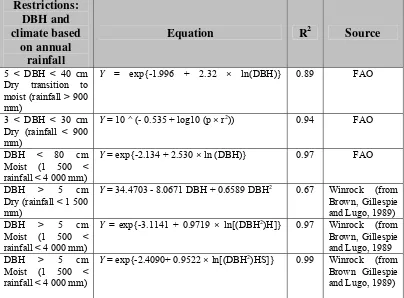
>4000 mm rain/year and no dry season). Table 2.1 depicts the regression models
for estimating biomass of tropical trees based on rainfall climatic zone, as the
research result conducted by Brown, Gillespie and Lugo (1989) in MacDicken
(1997).
The linear regression equation approach requires the selection of the
regression equation that is best adapted to the conditions in the study area. Linear
regression models have been fitted to data in various situations of variable site and
ecological conditions globally.
Table 2.1 Biomass regression equations for biomass estimation of tropical trees.
Climate type based on annual rainfall
Equation R2 Adjusted
Dry (<1500 mm) Y=34,4703-8,0671 D + 0.6589D2 0.67
Y=38,4908-11,7883D+1.1926D2 0.78
Y=exp[-3,1141+0,9719 ln (D2H)] 0.97
Y=exp[-2,4090+0,9522 ln (D2HS)] 0.99
Moist (1500-4000 mm)
H=exp[1,0701+0,5677 ln D)] 0.61
Y=13,2579-4,8945 D 0.90
Y=exp[-3,3012+0,9439 ln (D2H)] 0.90
Wet (>4000 mm)
H=exp[1,2017+0,5627 ln D] 0.74
Where: Y = Biomass/plant (kg)
D = Diameter at Breast height (cm) H = Height (m)
Table 2.2 Estimation of tropical forests biomass using regression equations of biomass as a DBH function.
Restrictions: DBH and climate based
on annual rainfall
Equation R2 Source
5 < DBH < 40 cm Dry transition to moist (rainfall > 900 mm)
Y = exp{-1.996 + 2.32 × ln(DBH)} 0.89 FAO
3 < DBH < 30 cm Dry (rainfall < 900 mm)
Y = 10 ^ (- 0.535 + log10 (p × r2)) 0.94 FAO
DBH < 80 cm Moist (1 500 < rainfall < 4 000 mm)
Y = exp{-2.134 + 2.530 × ln (DBH)} 0.97 FAO
DBH > 5 cm Dry (rainfall < 1 500 mm)
Y = 34.4703 - 8.0671 DBH + 0.6589 DBH2 0.67 Winrock (from
Brown, Gillespie and Lugo, 1989) DBH > 5 cm
Moist (1 500 < rainfall < 4 000 mm)
Y = exp{-3.1141 + 0.9719 × ln[(DBH2)H]} 0.97 Winrock (from
Brown, Gillespie and Lugo, 1989 DBH > 5 cm
Moist (1 500 < rainfall < 4 000 mm)
Y = exp{-2.4090+ 0.9522 × ln[(DBH2)HS]} 0.99 Winrock (from
Brown Gillespie and Lugo, 1989)
Source: FAO document “Assessing carbon stocks and modeling win-win scenario of carbon sequestration”
Where: p = 3.1415927 r = radius (cm)
DBH = diameter at breast height (cm) H = height (m)
BA = J × r2
S = wood density (0.61)
The work done by Brown, Gillespie and Lugo (1989) and FAO (1997) on
estimation of above ground biomass of tropical forests using regression equations
of biomass as a function of DBH is central to the use of this approach. DBH is
used in estimating the amount of wood volume is a stand of trees (White 1998 in
FAO). Some of the equations reported by Brown, Gillespie and Lugo (1989) have
become standard practice because of their wide applicability. Table 2.2 presents a
restrictions placed on each method.
2.1.3.3 Approach 3: Biomass Estimation from GIS Modeling
The approach for estimating biomass density based on modeling method
with GIS (Geographic Information System) technology uses various existing
digital data bases and maps of reliable inventories, population, density, climate,
vegetation, ecofloristic zones, soils and topography. This method was developed
as a means to extrapolate reliable inventory data that is generally limited in area
coverage to biomass density estimates at larger scales such as continents (Brown,
1997).
Forest biomass density has been modeled in a multi-stage approach using
GIS software packages and a variety of spatial and statistical data base. For
estimating forest biomass density using GIS, the present distribution of forest
biomass density was assumed to be based on the potential amount that the
landscape can support under prevailing environmental conditions, and the
cumulative impact of human activities on forests that reduce it biomass density.
Many spatial data layers have been developed from existing data bases or were
prepared by specialist (FAO, 1993 in Brown 1997). These data layers were
entered into a GIS and processed according to specifications of the model.
The first step in this analysis was to estimate a potential biomass density
(PBD) for forests. This was accomplished by first developing an index of
potential biomass density based on climatic, edaphic and topographic factors. The
potential biomass density map was masked with a forest map, produced by
reclassifying all the forest classes of the vegetation maps into one forest class. The
based on overlaying the following GIS data layers:
PBI= climatic index + precipitation + soil (texture, depth, slope) + topography
Each of these factors was spatially represented by a numerical scale
whose values were ranked according to how the particular factor affected forest
biomass. The digital maps were overlain according to the above model and the
results calibrated and validated using existing forest inventories for mature forests.
The final step was to add the influence of all human activities that result
in a reduction of biomass of forests. This step was accomplished by using the
biomass estimates from reliable forest inventory data. The first step was to
calculate degradations ratios, defined here as biomass density estimations from the
inventories (representing all forests of a sub-national unit) divided by the potential
biomass for all forest in the same sub-national unit.
2.1.3.4 Approach 4: Biomass Estimation with Field Studies and Remote Sensing
A more comprehensive and reliable approach for estimating biomass
change is to combine a new field studies with analysis of high resolution remote
sensing imagery. The remote sensing efforts would be used to delineate forests
into various distinct biomass strata. Then using statistical design, permanent plots
in these forest strata could be established. For estimating biomass directly, stand
tables are sufficient with use of the generic biomass regression equations. At least
two measurements on permanent plots are needed to estimate biomass change.
These measurements should preferably be a minimum of 5 year apart, particularly
2.1.4 Carbon Stock
Carbon stock is the amount of carbon which is stored in the biomass
component and necromas above and below soil surface (soil organic content, plant
root and microorganism) per unit area of land (Hairiah et al., 2003). The unit is in
Mg ha-1 (mega gram per ha = ton per ha). One of the important functions of the
forest is as the terrestrial carbon stock, because carbon is stored in the form of
vegetation biomass.
2.1.5 Carbon stock measurement
2.1.5.1 Aboveground C: Allometric relation for trees
A major proportion of the C and nutrients in terrestrial ecosystem is
found in the tree component. To reduce the need for destructive sampling,
biomass can be estimated from an easily measured property such as stem diameter
at a specified height, by using an allometric equation. Such equations exist for
many forest types and a small number are species specific (Hairiah et al., 2001).
Destructive measurement of trees (cutting down and weighting) to generate
allometric equations, which have high precision needs a lot of labor and time, but
when it is done it can be applied to other tree species in the same forest area. A
substantial number of allometric equations have been developed for various
climatic zones, forest types and tree species (Brown, 1997), using a variety of
algebraic forms and parameter values.
The calculation of carbon stock as biomass consists of multiplying the
total biomass by a conversion factor that represents the average carbon content in
biomass. It is not practically possible to separate the different biomass
the biomass component. Therefore, the coefficient of 0.55 for the conversion
biomass to C, offered by Winrock (1997), is generalized here to conversions from
biomass to carbon stock:
C = 0.55 × biomass (total)
This coefficient is widely used internationally, thus it may be applied on
a project basis. The results may be displayed in a similar fashion to total biomass.
Carbon stocks of natural forests in Southeast Asia Using GIS, Brown et
al., (1993) estimated that in 1980 the Winrock (1997) average C density of
tropical forests in Asia was 144 ton C/ha in biomass and 148 ton C/ha in soils (up
to 100 cm), which corresponds to total estimates of 42 and 43 Pg C for the whole
continent, respectively. It was noted that C densities and pools in vegetation and
soil varied widely by eco-floristic zone and country. Actual biomass C densities
range from less than 50 to more than 360 ton C/ha with most forests having 100 -200 ton C/ha.
A similar study reported an average maximum aboveground biomass C
stock in forest lands in tropical Asia of 185 ton C/ha with a range of 25 to more
than 300 ton C/ha. Palm et al. (1993), as reported by Houghton (1991), showed
that the forests in tropical Asia have C densities between 40-250 ton/ha and 50 -120 ton/ha in vegetation and soils, respectively. Southeast Asian forests have an
aboveground biomass range of 50-430 ton/ha (25-215 ton C/ha) and >350-400 ton/ha (175-200 ton C/ha) before human incursion (Brown et al., 1991). For national GHG inventories, the IPCC (1997) recommends a biomass density
default value of 275 ton/ha (or 138 ton C/ha) for wet forests in Asia.
Southeast Asian countries. Indonesian forests have been estimated to have a C
density ranging from 161-300 ton C/ha in aboveground biomass (Murdiyarso and Wasrin, 1995), 150-254 ton C/ha in above ground biomass and upper 30 cm of soil (Hairiah, et al., 2000) and 390 ton C/ha in above ground biomass and below
ground pools (Hairiah and Sitompul, 2000).
2.1.5.2 Below ground C: root biomass
Root are an important part of the C cycle because they transfer large
amounts of C directly in to the soil, where it may be stored for long time. Most of
below-ground biomass of forest is contained in coarse roots (>2mm diameter), but
most of that of annual crops is allocated to fine roots. Similar to approach for
above ground biomass via allometric relations based on stem diameter, the below
ground biomass can be estimated from the proximal roots at the stem base. The
theoretical basis for this relationship is found in the fractal branching properties of
root system (van Noordwijk and Purnomosidhi, 1995).
2.1.5.3 Belowground C: Soil Organic Matter
Soil organic matter content at any point in time is the result of organic
inputs and the past rates of decomposition, as determines by inherent properties of
the soil and the vegetation or land use system of the site. There are large
differences in C storage capacity of soil related to: soil texture, landscape position
and degree of drainage, mineralogy and physical disturbance.
2.2 Remote Sensing
Remote sensing is the science and art of obtaining information about an
object, area, or phenomenon through the analysis of data required by a device that
(Lillesand and Kiefer, 2001).
2.2.1 Remote Sensing Application in Forestry
Application of remote sensing to sustainable forest management are
presented in four categories that include classification of forest cover type,
estimation of forest structure (inventory mapping), forest change detection and
forest modeling. The inventory mapping of forest covers the measurement of
cover, age, DBH, height, biomass, volume and growth (Franklin, 2001). Users in
many countries adopt the remote sensing in many applications in forestry. These
applications include forest cover type characterization, determination of forest
stand conditions and forest health, site characterization and fire monitoring
(Wynne and Carter, 1997). In India use remote sensing for plantation inventory
and monitoring, timber volume estimation, species identification, estimation of
biomass and productivity and biodiversity monitoring (Raa et al., 1997).
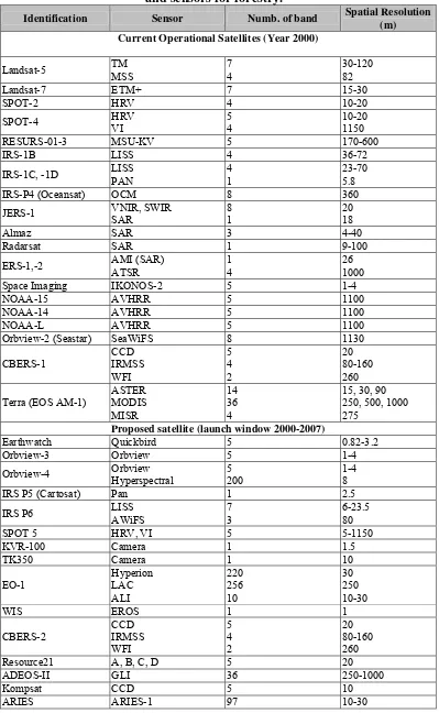
Table 2.3 listed the most system provide observation from a single
sensors in either optical (e.g. Landsat, SPOT, IRS) or microwave (e.g. Radarsat,
ERS-1) portion of the spectrum; occasionally a satellite will carry both types of
sensor (e.g. ALMAZ). A few systems have thermal detectors or other sensors as
part of the package but, in essence, the choice of a platform/sensor package in
support of forestry applications has been limited in the past to a few satellites with
quite similar characteristic in the optical or microwave portions of the spectrum
Table 2.3 Characteristic of selected existing and proposed satellite platforms and sensors for forestry.
Identification Sensor Numb. of band Spatial Resolution
(m) Current Operational Satellites (Year 2000)
Landsat-5 TM
MSS
7 4
30-120 82
Landsat-7 ETM+ 7 15-30
SPOT-2 HRV 4 10-20
SPOT-4 HRV
VI
5 4
10-20 1150
RESURS-01-3 MSU-KV 5 170-600
IRS-1B LISS 4 36-72
IRS-1C, -1D LISS
PAN
4 1
23-70 5.8
IRS-P4 (Oceansat) OCM 8 360
JERS-1 VNIR, SWIR
SAR
8 1
20 18
Almaz SAR 3 4-40
Radarsat SAR 1 9-100
ERS-1,-2 AMI (SAR)
ATSR
1 4
26 1000
Space Imaging IKONOS-2 5 1-4
NOAA-15 AVHRR 5 1100
NOAA-14 AVHRR 5 1100
NOAA-L AVHRR 5 1100
Orbview-2 (Seastar) SeaWiFS 8 1130
CBERS-1 CCD IRMSS WFI 5 4 2 20 80-160 260
Terra (EOS AM-1)
ASTER MODIS MISR 14 36 4
15, 30, 90 250, 500, 1000 275
Proposed satellite (launch window 2000-2007)
Earthwatch Quickbird 5 0.82-3.2
Orbview-3 Orbview 5 1-4
Orbview-4 Orbview
Hyperspectral
5 200
1-4 8
IRS P5 (Cartosat) Pan 1 2.5
IRS P6 LISS
AWiFS
7 3
6-23.5 80
SPOT 5 HRV, VI 5 5-1150
KVR-100 Camera 1 1.5
TK350 Camera 1 10
EO-1 Hyperion LAC ALI 220 256 10 30 250 10-30
WIS EROS 1 1
CBERS-2 CCD IRMSS WFI 5 4 2 20 80-160 260
Resource21 A, B, C, D 5 20
ADEOS-II GLI 36 250-1000
ALOS VSAR 1 10
AVNIR-2 5 2.5-10
Envisat-1 ASAR 1 30,150
MERIS 15 300,1200
Radarsat-2 SAR 1 6.25-500
LightSAR SAR 4 3-100
XSTAR XSTAR 10+ 20
NEMO (HRST) AVIRIS 211 5-30
EROS-A1,-A2 Pan 1 1.5
EROS-B1 Pan 1 0.82
Aqua(EOS PM-1) MODIS 36 250-1000
Resource21 CIRRUS 6 10-100
M11 MTI 15 5
NOAA-M,-N AVHRR 5 1100
Source: Adapted from Morain, 1998; Chen, 1998; Glackin, 1998; Stoney and Hughes, 1998; Dowman,
1999; Barnsley, 1999; Estes and Truelove, 1999. http://rs320h.ersc.edu/ERSCin Jensen, 2000
2.2.2 Remote Sensing for Aboveground Biomass Estimation
Remotely sensed data are understood here as the data generated by
sensors from a platform not directly touching or in close proximity to the forest
biomass. Therefore, these data comprise images sensed from both aircraft and
satellites. Remote-sensing imagery can be extremely useful, particularly where
validated or verified with ground measurements and observations (i.e. “ground
truth”). Remote-sensing images can be used in the estimation of aboveground
biomass in at least three ways (FAO document, 2000)
• Classification of vegetation cover and generation of a vegetation type map.
This partitions the spatial variability of vegetation into relatively uniform
zones or vegetation classes. These can be very useful in the identification
of groups of species and in the spatial interpolation and extrapolation of
biomass estimates.
• Indirect estimation of biomass through some form of quantitative
relationship (e.g. regression equations) between band ratio indices (NDVI,
digital numbers per pixel, with direct measures of biomass or with
parameters related directly to biomass, e.g. leaf area index (LAI).
• Partitioning the spatial variability of vegetation cover into relatively
uniform zones or classes, which can be used as a sampling framework for
the location of ground observations and measurements.
2.2.3 Different Satellite Images in Biomass and C-Stock Estimation
Landsat TM satellite image was used for regional biomass mapping in
Madhav National Park-India (Ravan and Roys, 1996). In estimating the biomass,
the ground based method was applied. It means that for estimating total above
ground biomass (dry weight) natural ecosystem was divided into three
components: trees, shrubs and grasses. Ground sampling was carried out by lying
sample plots in homogenous vegetation strata. The quantitative measurements of
plant parameters in these plots include girth at breast height (for trees) and height
of individual plant. The result indicates that there is a significant relationship with
spectral responses. These relationships have seasonal dependency in varying
phonological conditions. The relationships are strongest in visible bands and
middle infrared bands. However, spectral biomass models developed using middle
infrared bands would be more reliable as compared to the visible bands as the
later spectral regions are less sensitive to atmospheric changes. It was observed
that brightness and wetness parameters show very strong relationship with the
biomass values. Multiple regression equations using brightness and wetness
isolates have been used to predict biomass values. The model used has correlation
coefficient of 0.77. Percent error between observed and predicted biomass was
spectral response modeling approaches were compared and showed similarity
with the difference of only 4.69%. The result indicates that satellite remote
sensing data provide capability of biomass estimation (Ravan and Roys, 1996).
2.2.4 Remote Sensing Estimation of LAI
Leaf Area Index (LAI) is ratio of the total area of all leaves on a plant to
the area of ground covered by the plant (m2/m2). LAI is defined as one sided green
area per unit ground area in broadleaf canopies and as projected needle leaf area
in coniferous canopies. LAI provides a simple measure of plant canopy density.
LAI varies from less than 1 in desert to greater than 10 over tropical rain forest.
Therefore, changes in LAI can also be indicative of land cover change (Nemani et
al, 1996)
LAI describes a fundamental property of the plant canopy in its
interaction with the atmosphere. It is an important structural parameter for
quantifying the energy and mass exchange characteristic of terrestrial ecosystem
such as photosynthesis, respiration, carbon, and nutrient cycle, and rainfall
interception (Gong et al. 2003).
In some remote sensing studies, LAI is expressed as a one-sided ration of
leaf area to projected ground area; in others, all sided LAI is measured. LAI is an
important structural attribute of forest ecosystem because of its potential to be a
measure of energy, gas and water exchanges. For example, physiological
processes such as photosynthesis, transpiration and evapo-transpiration are
functions of LAI (Pierce and Running 1988). Accordingly, LAI and forest cover
type are the two critical inputs available from remote sensing that are required to
landscape (Running et al., 1986; Bonan, 1993; Peterson and Waring, 1994). LAI
may be estimated at a variety of scales and with many different instrument and
techniques (Chen and Cihlar, 1995). In the field, LAI can be estimated using
litterfall sampling, sapwood allometric and light interception observation and all
of labor-intensive and impractical for larger stands and landscapes (Smith et al.,
1991; Fassnacht et al., 1994).
Remote sensing estimation of LAI is based on the knowledge that green
leaves interact selectively with solar radiation (Jasinski, 1996). Much of the
near-infrared energy is reflected by foliage (Knipling, 1970; Gausman, 1977); much of
the visible energy (dominated in the red portion of the spectrum) is absorbed by
photosynthesis pigments (Waring et al., 1995). Vegetation indices such as NDVI
or the simple ration (SR) can be used to capture the way in which red and near-IR
reflectance differ in single measure. The common approach of LAI estimation is
empirical and semi-empirical modeling; the same approach discussed above,
involving correlation of spectral indices with field estimates and the extension of
such estimates over large areas with regression (Curran et al., 1992; Peddle et al.,
1999; Wulder et al., 1996) or canopy reflectance model (Huemmrich and Goward,
1997).
2.2.5 Vegetation Indices
A vegetation index is a quantitative measure used to measure biomass or
vegetative vigor, usually formed from combinations of several spectral bands,
whose values are added, divided, or multiplied in order to yield a single value that
indicates the amount or vigor of vegetation. The simplest form of vegetation index
this ratio will be high due to the inverse relationship between vegetation
brightness in the red and infrared regions of the spectrum.
A vegetation index (VI) was introduced as a simple remote sensing tool
for over 25 years. Vegetation indices have been used for many years of increasing
importance in the field of remote sensing. VI was a number that is generated by
some combinations of remote sensing band and may have some relationship to the
amount of vegetation in a given image pixel. Remote sensing devices operated in
the green, red and near infrared regions of the electromagnetic spectrum, they act
as sensitive discriminators of variations in radiation output that measure both
absorption and reflectance effects associated with vegetation.
There are more than 20 vegetation indices in use are summarized in
Table 2.4. Many are functionally equivalent (redundant) in information content
(Perry and Lautenschlager, 1984), while some provide unique biophysical
information (Qi et al., 1995). It is useful to review the historical development of
the main indices and provide information about recent advances in index
development.
Cohen (1991) suggests that the first true vegetation index was the simple
ratio (SR), which is the near-infrared (NIR) to red reflectance ratio described in
Birth and McVey (1968)
d NIR SR
Re =
Rouse et al., (1974) developed what is now called the generic
Table 2.4 Selected Remote Sensing Vegetation Index (Jensen 2000).
Vegetation Index Equation
Simple Ratio (SR)
RED NIR
SR=
Normalized Difference Vegetation Index
(NDVI) NIR red
red NIR NDVI + − =
Infrared Index (II)
5 4 5 4 MidIRTM NIRtm MidIRtm tm NIR II + − = Perpendicular Vegetation Index 2 ) 4 2 2 2
4 0.149 ) (0.355 0.852 )
355 . 0
( mms mms mms mms
PVI = − + −
Greenness Above Bare
Soil (GRABS) GRABS=G−0.09178B+5.58959
Moisture Stress Index (MSI) 4 5 TM TM NIR MidIR MSI =
Leaf Relative Water
Content Index (LWCI)
[
[
]
]
ft ft TM TM TM TM MidIR NIR MidIR NIR LWCI 5 4 5 4 1 log ) ( 1 log − − − − − − = MidIR Index 7 5 TM TM NIR MidIR MidIR=
Soil Adjusted Vegetation Index (SAVI) and Modified SAVI (MSAVI) L red NIR red NIR L SAVI + + − +
= (1 )( )
Atmospherically
Resistant Vegetation
Index (ARVI) ⎟⎟⎠
⎞ ⎜⎜ ⎝ ⎛ + − = rb nir rb nir p p p p ARVI * * * * Soil and Atmospherically Resistant Vegetation Index (SARVI) L p p p p SARVI rb nir rb nir + + − = * * * * Enhanced Vegetation
Index (EVI) (1 )
* * * * * 2 1 L L p C p C p p p EVI blue blue nir red nir + + − + − =
2.2.5.1 Simple Ratio (SR)
Cohen (1991) suggest that the first true vegetation index was the Simple
Ratio (SR), which is the near-infrared (NIR) to red reflectance ratio described in
Birth and McVey (1968);in Jensen (2000)
NIR RED
2.2.5.2 Normalized Difference Vegetation Index (NDVI)
NDVI (Normalized Difference Vegetation Index) is one of the ratio
indices that respond to changes in amount of green biomass, chlorophyll content
and canopy water stress. The healthy and dense vegetation show a large NDVI.
Areas covered with clouds, water and snow yield negative index value while areas
covered with rock and bare soil result in vegetation indices near zero.
The pigment in plant leaves, chlorophyll strongly absorbs visible light
(from 0.4 to 0.7 µm) for use in the photosynthesis. The cell structure, on the other
hand, strongly reflects near infrared light (from 0.7 to 1.1 µm). The more leaves a
plant has, the more these wavelengths of light are affected, respectively.
By comparing visible and infrared light, scientist measures the relative
amount of vegetation. Healthy and dense vegetation absorbs most of the visible
light that hits it. Unhealthy and sparse vegetation reflects more visible light and
less near infrared. Mathematically, NDVI is written as:
RED NIR
RED NIR
NDVI
+ − =
The actual difference between the reflected sunlight from the red part of
the spectrum and the reflected energy in the near infrared gives a qualitative
measure for photosynthesis activity. NDVI value range from minus one (-1.0) to
plus one (+1.0) and are unitless (Wunderle et al, 2003).
NDVI is a good indicator of the ability for vegetation to absorb
photosynthetically active radiation has been widely used by researcher to estimate
green biomass, LAI and patterns of productivity. The main advantages of the use
extensive area coverage and high temporal frequency of remote sensing data
(Hess T. et al, 1996).
Environmental factors such as soil geomorphology and vegetation all
influence NDVI values should be taken into account. NDVI can be effective in
predicting surface properties when vegetation canopy is not to dense or too sparse.
If a canopy is to sparse, background signal (e.g. soil) can change NDVI
significantly. Depending on the vegetation coverage, dark soil enhances the NDVI
(Wunderle et al, 2003). If the canopy too dense, NDVI saturates because red
reflectance does not change much, but NIR reflectance still increase when the
canopy become denser.
A few studies have attempted to predict forest biomass using the
relationships between reflectance and crown closure, crown size, and species. In
Japan, Lee and Nakane (1997) estimated biomass with a variety of vegetation
indices obtained from Landsat TM Imagery in predominantly deciduous stands
(comprised of Quercus serrata, Catanea crenata and Carpinus laxiflora), pine
(Pinus densiflora) forests, and Japanese cedar (Cryptomeria japonica) plantation.
The NDVI was best in predicting biomass in the pine stands (R value was 0.85).
In the deciduous and cedar plantations, the difference between band 5 and 7
(called the DVI) was the best predictor (R value=-0.83 for cedar, and +0.80 for
deciduous stands) (Table 2.5).
Table 2.5 The relationship between Landsat TM-Based DVI (Difference between bands 5 and 7) and biomass in 33 stands of deciduous and cedar
plantation in Japan.
Stand Type R Value
The sign of the relationship between biomass and DVI changed in the
cedar plantations compared to the deciduous stands. The cedar plantation was
comprised of stands with the relatively similar age classes. Trees were a uniform
diameter and canopy height. The spectral response was more scattered due to the
sharp, triangular cedar crown. The DVI was thought to be more sensitive to
vegetation density than to leaf moisture content and color. The changes in the
relationship among the species were attributed to the influences of different
shadowing and leaf biomass.
Biomass distribution in forest ecosystem is a function of vegetation type,
its structure and site condition. Ground based sampling in functional homogenous
vegetation categories is an approach which has found acceptability in the recent
past (Shute and West 1982)
The NDVI has been shown to be useful in estimating vegetation
properties, many important external and internal influence restrict its global
utility.
2.3 Empirical Modeling
Empirical models are based on statistical analysis of observed data, and
these are usually applicable only to the same conditions under which the
observations were made. An empirical model is based only on data and is used to
predict but not to explain the process of system. An empirical model consists of a
function that captures the trend of the data. Data are essential for an empirical
model.
Sometimes with a derived model, it might be difficult or impossible to
modeling (EM) offered both a broad foundational perspective on computing and a
novel practical approach to modeling. Central to the EM perspective was an
emphasis on the power of the computer to represent state in particular, state that
was easily interpretable. Adopting a broad concept of what constituted a computer
any reliable, interpretable, state changing device led to a view in which the
context for computing (e.g