arXiv:0711.0275v1 [math.AP] 2 Nov 2007
DOMAINS : NEUMANN BOUNDARY CONDITIONS
by
Nicolas Burq & Fabrice Planchon
Abstract. — We prove that the defocusing quintic wave equation, with Neumann boundary
conditions, is globally wellposed onHN1(Ω)×L2(Ω) for any smooth (compact) domain Ω⊂
R3. The proof relies on one hand onLpestimates for the spectral projector ([13]), and on
the other hand on a precise analysis of the boundary value problem, which turns out to be much more delicate than in the case of Dirichlet boundary conditions (see [3]).
1. Introduction
Let Ω ∈ R3 be a smooth bounded domain with boundary ∂Ω and ∆N the Laplacian acting on functions with Neumann boundary conditions. In [3] (with G. Lebeau), we derived Strichartz inequalities for the wave equation fromLp estimates for the associated spectral projector, obtained recently by H. Smith and C. Sogge [13]. As an application we obtained global well-posedness for the defocusing energy critical semi-linear wave equation (with real initial data) in Ω, with Dirichlet boundary conditions. Here we are interested in the similar question for the Neumann case,
(1.1) (∂
2
t −∆)u+u5 = 0, inRt×Ω u|t=0 =u0, ∂tu|t=0 =u1, ∂nu|Rt×∂Ω= 0.
Here and thereafter,∂ndenotes the normal derivative to the boundary∂Ω. Equation (1.1) enjoys the usual conservation of energy
E(u)(t) = Z
Ω
|∇u|2(t, x) +|∂
tu|2(t, x)
2 +
|u|6(t, x) 6
dx=E(u)(0) =E0.
LetHN1 denote the Sobolev space associated to the Neumann Laplacian. Our main result reads:
Theorem 1. — For any(u0, u1)∈HN1(Ω)×L2(Ω)there exists a unique (global in time)
solution u to (1.1) in the space
Remark 1. — Smith and Sogge’s spectral projectors results hold irrespective of Dirichlet or Neumann boundary conditions. As such, the local existence result will be obtained as in [3]. However, the non-concentration argument requires considerably more care, including non-trivial Lp estimates for the traces of the solutions on the boundary. We provide a self-contained proof of the specific estimates we need, which applies to our nonlinear equation. A different set of results in that direction was announced in [17] in a more general setting for linear wave equations.
Remark 2. — Using the material in this paper, it is rather standard to prove existence of global smooth solutions, for smooth initial data satisfying compatibility conditions (see [12]). Furthermore, our arguments apply equally well to more general defocusing non linearitiesf(u) =V′(u) satisfying
|f(u)| ≤C(1 +|u|5), |f′(u)| ≤C(1 +|u|)4.
Finally, let us remark that our results can be localized (in space) and consequently hold also for a non compact domain and in the exterior of any obstacle, and we extend in this framework previous results obtained by Smith and Sogge [12] for convex obstacles (and Dirichlet boundary conditions).
Fors≥0, let us denote byHNs(Ω) the domain of (−∆N)s/2. Finally, , we setA.B to meanA≤CB, whereC is an harmless absolute constant (which may change from line to line).
2. Local existence
The local (in time) existence result for (1.1) is a direct consequence of some recent work by Smith and Sogge [13] on the spectral projector defined by Πλ = 1√−∆N∈[λ,λ+1[.
Theorem A (Smith-Sogge [13, Theorem 7.1]). — Let Ω ∈ R3 be a smooth bounded domain and ∆ be the Laplace operator with Dirichlet or Neumann boundary conditions, then there exists C >0 such that for any λ≥0,
(2.1) k1√
−∆∈[λ,λ+1[ukL5(Ω).λ 2 5kuk
L2(Ω).
From which we derive Strichartz estimates, which are optimal w.r.t scaling.
Theorem 2. — Assume that for some 2≤q <+∞, the spectral projectorΠλ satisfies
(2.2) kΠλukLq(Ω).λδkukL(Ω).
Then the solution to the wave equation v(t, x) =eit√−∆Nu
0 satisfies kvkLq((0,2π)t×Ωx) .ku0k
Hδ+ 12 −1
q N
.
The proof given in [3] applies verbatim and we therefore skip it.
Proposition 2.1. — If u, f1, f2 satisfy
then
(2.3) kuk
L5((0,1);W103,5
N (Ω))
+kukC0((0,1);H1
N(Ω))+k∂tukC0((0,1);L2(Ω))
≤Cku0kH1
N(Ω)+ku1kL2(Ω)+kf1kL1((0,1);L2(Ω))+kf2kL54((0,1);W107,54(Ω))
.
Furthermore, (2.3)holds (with the same constantC) if one replaces the time interval(0,1)
by any interval of length smaller than 1.
Remark 3. — Notice that by Sobolev embedding and trace lemma, one has
(2.4) kukL5((0,1);L10(Ω))+ku|∂Ωk
L5((0,1);L203 (∂Ω)) .kuk
L5((0,1);W103 ,5
N (Ω))
,
which will play a crucial role in the non-concentration argument.
Corollary 2.2. — For any initial data(u0, u1)∈HN1(Ω)×L2(Ω), the critical non linear
wave equation (1.1)is locally well posed in
XT =C0([0, T];HN1(Ω))∩Lloc5 ((0, T);L10(Ω))×C0([0, T];L2(Ω))
(globally for small norm initial data).
We refer to Appendix A for a proof of Proposition 2.1. The proof of Corollary 2.2 pro-ceeds by a standard fixed point argument with (u, ∂tu) in the spaceXT with a sufficiently small T (depending on the initial data (u0, u1)). Note that this local in time result holds irrespective of the sign of the nonlinearity.
Finally, to obtain the global well posedness result for small initial data, it is enough to remark that if the norm of the initial data is small enough, then the fixed point can be performed in XT=1. Then the control of theH1 norm by the energy (which is conserved along the evolution) allows to iterate this argument indefinitely leading to global existence. Note that this result holds also irrespective of the sign of the nonlinearity because for small H1 norms, the energy always control the H1 norm.
3. Global existence
It turns out that our Strichartz estimates are strong enough to extend local to global
existence for arbitrary (finite energy) data, when combined with trace estimates and non concentration arguments.
Before going into details, let us sketch the proof. Remark that iff =u5, we can estimate
(3.1)
ku5k
L54((0,1);L3017(Ω))≤ kuk
4
L5((0,1);L10(Ω))kukL∞
((0,1);L6(Ω)),
k∇x(u5)kL5
4((0,1);L109 (Ω))= 5ku 4
∇xukL5
4((0,1);L109(Ω)) ≤5kuk4L5((0,1);L10(Ω))kukL∞
((0,1);H1(Ω)). Interpolating between these two inequalities yields
(3.2) ku5k
L54((0,1);W107,54(Ω)).kuk 4
L5((0,1);L10(Ω))kuk 3 10 L∞
((0,1);L6(Ω))kuk 7 10 L∞
Following ideas of Struwe [14], Grillakis [5] and Shatah-Struwe [10, 11], we will localize these estimates on small light cones and use the fact that theL∞
t ;L6x norm is small in such small cones. Unlike with Dirichlet boundary conditions, we cannot hope to have a good control of the H1 norm of the trace of u on the boundary (this control is known to be false even for the linear problem), and it will require a more delicate argument to handle boundary terms.
3.1. The L6 estimate. — In this section we shall always consider solutions to (1.1) in
(3.3) X<t0 =C0([0, t0);HN1(Ω))∩Lloc5 ([0, t0);L10(Ω))×C0([0, t0);L2(Ω)).
Moreover, we assume these solutions to have energy bounded by a fixed constant (namely, E0). By a standard procedure, such solutions are obtained as limits in X<t0 of smooth solutions to the analog of (1.1) where the nonlinearity and the initial data have been smoothed out. Consequently all the subsequent integrations by parts will be licit by a limiting argument.
3.1.1. The flux identity. — By time translation, we shall assume later that t0 = 0. Let us first define boundary condition, there is no flux through∂ΩT
An integration by parts gives (see Rauch [9] or [12, (3.3’)]) Eloc(S) being a non-negative non-increasing function, it has a limit whenS→0−, and
(3.8) Flux(u, MS0) = lim
3.1.2. A priori estimate for traces. — We prove an priori estimate on finite energy so-lutions of (1.1), which is reminiscent of results obtained in [17] for variable coefficients linear wave equations. Observe that, unlike in the Dirichlet case, we don’t have any uni-form Lopatinskii condition, which prevents control of the gradient on the boundary. The following result will provide a substitute. It shows that even though (due to the failure of the uniform Lopatinskii condition), the H1 norm of the trace is known to be unbounded (at least for the linear equation), the integral on the boundary of a specific quadratic form (namely the so-called Q0 null form) remain bounded (see [17] for related results).
Proposition 3.1. — Letn(x)be the exterior unit normal vector to∂Ω,−ε < S < T ≤0,
Remark 4. — For the solution of thelinear wave equation,u= 0, taking the trace on the boundary∂Ω in (2.3) gives
(3.11) ku|∂Ω k
And interpolating between the two estimates in the l.h.s. of (3.11) gives
ku|∂ΩkL6((0,1)×∂Ω)≤C
ku0kH1
N(Ω)+ku1kL2(Ω)
As a consequence, one could infer that the u6 term in the r.h.s. of (3.10) is not the most important part of the estimate. However, we will not use this fact here and shall prove the estimate (3.10) as a whole
Lemma 3.2. — There exists a smooth vector field Z (depending on (t, x)) defined on a neighborhood of x0 in [−t0,0)×Ωsuch that
1. We have Z|∂Ω =∂n+τ where ∂n is the interior normal derivative to the boundary and τ is a vector field which is tangent to the boundary;
2. The restriction of Z to the sphere St={x∈Ω;|x|=−t} is tangent to that sphere.
Proof. — Performing a linear orthogonal change of variables, we can assume that ∂3 = ∂n(0), with n(0) the normal vector to ∂Ω at x = 0. We now build a vector field Z ∈ C∞(Ω;TΩ) (as such, it does not have a ∂t component) such that its restriction to∂Ω is
close to ∂n (which, in a neighborhood of x = 0, B(0, η), is essentially ∂3 up to an O(η) term).
Consider the half-spherex3= √
1−r2, withr2 =x2
1+x22. To define a vector fieldX in the zonex3 < 34 (thus multiplying by a cut-offφ(x) such thatφ= 0 forx >3/4 andφ= 1 forx <1/4), we setX=X1 =∂3forr <1/4; forr >3/4, we setX =X2 =∂3−r−1x3∂r. On the half-sphere, X will be tangent and pointing in the same direction as ∂3 (or ∂ν). Now, we may smoothly connect both zones and define X within the entire half-sphere: consider φ∈C0∞(−1/2,1/2) equal to 1 on (0,1/4) and
X=φ(x3)(φ(r)∂3+ (1−φ(r))(∂3− x3
r ∂r)).
Then one rescales (x3, r) to be (x3/t, r/t). Note that on thex3= 0 axis,X =∂3. We now set
Xt=φ(x3/t)(φ(r/t)X1(x/t) + (1−φ(r/t))X2)(x/t).
Remark that X1, X2, as previously defined, are time independent (and smooth in zones whereX 6= 0). The vector field Xt is tangent to the sphereSt by definition. However, it requires to be renormalized so that its component on the normal to the spatial boundary is one: definez(x)∈∂Ω to be the orthogonal projection to the (spatial) boundary, we set
Z = 1
Xt(z(x))·n(z(x)) Xt,
which is easily seen to satisfy all our requirements.
Now we define a smooth weight w(x), such that its restriction to the boundary ∂Ω is x·n(x), and such that |w(x)|=O(|r|2): w(x) =z(x)·n(z(x)) is such a weight.
To prove Proposition 3.1, we start with the following commutator estimate.
Proposition 3.3. — There existsC >0 such that
(3.12)
Z
KT S∩ΩTS
[(∂t2−∆), Z]u(t, x)·u(t, x)w(x)dxdt .|S|
2(E 0+E
2 3
0).
Proof. — We shall make a repeated use of the following
Lemma 3.4. — Consider a function a(x, t) such that
Then there exists C > 0 such that for any solution with energy E0, for all S, T s.t. −1≤S < T <0,
(3.13)
Z
KT S
a(x, t)u(x, t)∇x,tu(x, t)dxdt
.E23
0|S|2.
Proof. — We have
(3.14) Z
KT S
a(x, t)u(x, t)∇x,tu(x, t)dxdt
≤Z T
S |∇
x,tu(x, t)|2dxdt
1/2Z
KT S
|u(x, t)|6dxdt1/6Z KT
S
|a(x, t)|3dxdt1/3
.E12+16(u)|S|12+16
Z
KT S
|a(x, t)|3dxdt1/3
.(E0|S|)2/3 Z T
S
Z
|x|<−t
dxdt1/3 =CE 2 3
0|S|2,
which achieves the proof.
We now prove a second lemma which will immediately yield Proposition 3.3:
Lemma 3.5. — Assume that Q = Pijqij∂ij2 is a smooth (space-time) second order op-erator with real coefficients (qij)ij, 0≤i, j≤3, satisfying
(3.15) ∀i, j, ∀(x, t);|x| ≤ −t, t∈(−1,0), |∂x,tα qij(x, t)|.|t|1−|α|, |α| ≤2.
Moreover, assume that (recalling (3.5)for the definition of ν)
(3.16) T =X i,j
((ν·∂i)qij)∂j is a vector field which is tangent to MST;
then, for any solution with energy E0, and any −1≤S < T <0,
(3.17)
Z
KT S
Q(x, t, Dx,t)u(x, t)u(x, t)dxdt
.|S|2(E0+E
2 3
Proof. — We integrate by parts to be the inward normal vector to∂Ω, whiledρ(resp. dσ) is the induced measure onMT S (resp. ∂Ω).
The contribution ofI is dealt with using Lemma 3.4. Next,
II.kqi,jkL∞(KT
S)|S|E(u).|S|
2E 0.
The contribution ofDS in III is bounded (using H¨older inequality) by
(3.19) Z
We deal with the contribution of DT to III similarly. To bound the contribution of IV, we remark that according to our assumptions onQ, the vector field
1
is tangential toMT
S. As a consequence (using H¨older inequality),
It remains to bound the contributions of V in the right hand side of (3.18). Using the Neumann boundary condition, we can replace the vector fields ∂j by their tangential components ∂j −(∂j·n(x))n(x). In a coordinate system y in the boundary and abusing notation for ∂yi, we now have to compute
with eq satisfying the same estimates asq, namely (3.15). Integrating by parts gives (3.22)
where the first term in the right hand side appears when the derivative hits the coefficients while the second term comes from the contribution of the boundary of KST ∩∂ΩTS).
To conclude, we use the following
Lemma 3.6. — For any solution u and any S < T <0, we have
Proof. — Let us first conclude the proof of Lemma 3.5 assuming Lemma 3.6. To deal with the first term in the right hand side of (3.22), we use H¨older inequality and obtain (using the trace theorem and then Sobolev embedding on ∂Ω)
(3.24) |V.1|.
To deal with the second term in the right hand side of (3.22), we also use H¨older inequality and obtain (using Lemma 3.6)
(3.25) |V.2|.Z
which ends the proof of Lemma 3.5
Let us now prove Lemma 3.6. The idea is roughly to take benefit of the fact that the flux controls the H1 norm on the cone MT
S; consequently by trace theorems it controls the H1/2 norm of the restriction ofuon the intersection of the cone and the spatial boundary. Hence, by Sobolev’s theorem, it controls theL4 norm. However, the geometry of the cone becomes singular near t= 0 and we have to be careful when implementing this idea. For this we decompose the time interval (S, T) into a union of dyadic intervals
For each integral, we perform the change of variables
is a smooth family of hypersurfaces of the cone (included in the smooth part of the cone corresponding to{t∈(1,1/2)} and consequently, the trace theorem applies with uniform constants; tracking the change of variables yields
ku
Summing the pieces back provides the desired estimate.
Back to proving Proposition 3.3, one may easily see that the coefficients of the second order operatorw(x)[, Z] satisfy the decay conditions of Lemma 3.4 and 3.5. We are left with (3.16): from decomposing the Laplacian in polar coordinates, the first order term (r−1∂r) is harmless, and so is the angular part. Then, ifA=∂t2−∂r2 = (∂t+∂r)(∂t−∂r),
we may return to the proof of Proposition 3.1 and perform integration by parts with the
operator in (3.26). Denote byD= ΩT
S ∩KST the space-time domain of integration. Its boundary∂D will be the reunion of two time slices, DT ∩Ω and DS∩Ω, one space slice
Leaving aside the first term, we compute the remaining term, namely Z
D
w(x, t)uZu dxdt.
We will apply Green’s second identity: recall that over 4-dimensional domains V, with ν∂V the outward normal to the boundary,
regains the lost factor S. The first term is no worse: one loses both factors S in deriving w twice, but on the other hand we get
Z
Dt
u2dx≤( Z
Dt
dx)23(
Z
Dt
u6dx)13 .S2E(u) 1 3,
since the volume of the ball Dt is t3 which produces the S2 factor. The middle term is, after substitution,
Z
D
w(x)Zu(x, t)(−u5)dxdt,
which may be added to the term we left in (3.27), to get
(3.29) 4 Z
D
(Zu)u5w(x)dxdt= 2 3
Z
D
Z(u6)w(x)dxdt
=−2 3
Z
D
u6Z(w)dxdt−2 3
Z
∂ΩT S∩KST
u6wdσ,
as Z is tangent to both the time slices and the cone (hence, the boundary contributions of these regions vanish). Recalling thatZ(w) =O(S),
Z
KT S×Ω
u6Zw(x)dxdt.S2E(u),
and we collect a term
(3.30) −2
3 Z
∂ΩT S∩KST
u6wdσ,
for later use.
We are now left with a space-time boundary term J coming from our application of (3.28), which is a difference of two terms
(3.31) J = Z
∂D
(uw)N ·
∂t −∇
Zu−Zu N·
∂t −∇
(uw) =J1−J2.
Here N is the outward normal derivative to the boundary∂D. The second termJ2 splits itself in three sub-terms.
– The first two are boundary terms on MST ∩Ω and DS ∪DT. The cone term is controlled by S2 times the flux, as one has only tangential derivatives on u (either Z or L=√2−1(∂t−∂r)). The time-slice terms are similarly controlled byS2 times the energy.
– The last one is
Z
∂ΩT S∩KST
uZu∂nw+wZu∂nu dσdt,
We are thus left withJ1, which we split again in three terms
J1 = Z
MT S
wu(LZu)dρ
+ Z
DT∩Ω
wu ∂tZu dx−
Z
DS∩Ω
wu ∂tZu dx
+ Z
KT S∩∂ΩTS
(∂nZu)uw dσdt
= K1+K2+K3.
Consider K3: we chose Z such that Z|∂Ω =∂n+τ, where τ is a tangent vector field to ∂Ω, so that
K3 = Z
KT S∩∂ΩTS
uw ∂n2u+wu[∂n, τ]u dσdt
= Z
KT S∩∂ΩTS
uw(∂t2−∆tan)u+u6w dσdt+ Z
KT S∩∂ΩTS
wu[∂n, τ]u dσdt.
We integrate by parts, to get Z
KT S∩∂ΩTS
uw(∂t2−∆tan+u4)u dσdt= Z
KT S∩∂ΩTS
(|∇tanu|2− |∂tu|2+u6)w dσdt
+ Z
KT S∩∂ΩTS
u∂tanu(ηw+∂tanw dσdt+B,
whereB is the boundary term to be specified below. The second term can be dealt with as in (3.20): η is the coefficient in [∂n, τ] which is tangent again (certainly, at least, when applied tou thanks to∂nu= 0 !). Now,
(3.32) B =
Z
∂ΩT S∩MST
wu N2·
∂t −∇tan
u dσ2,
whereN2 is the normal to∂Ω∩KST in∂Ω anddσ2 the induced (2D) measure; we leaveB for later treatment.
Adding the first term and the term (3.30), we get the left-handside of (3.10), namely Z
KT S∩∂ΩTS
(|∇tanu|2− |∂tu|2+ u6
3 )w dσdt
We now return toK2, writing (with an obvious abuse of notation for the domains)
K2 = Z
DT\DS
w(u[Z, ∂t]u−∂tuZu)dx
+ Z
(DT\DS)∩∂Ω
wu(N ·Z)∂tu dσ
+ Z
(DT\DS)∩MST
The last term vanishes, as Z is tangent to MST. The first one is controlled byS2E0. We collect the second one, denoted by M, for later treatment: recalling that on that part of ∂D,N =−∂n, we haveZ·N =−Z·∂n=−1 and
M =− Z
(DT\DS)∩∂Ω
wu∂tu dσ.
We now return to K1:
K1 = Z
ΩT S∩MST
wu[L, Z]u dρ
+ Z
ΩT S∩MST
wu ZLu dρ.
The commutator between two tangent vector fields is tangent, hence the fist term is controlled through the flux like in (3.20). By integration by parts, the second term is
− Z
Ω∩MT S
Z(wu)Lu dρ+ Z
∂(Ω∩MT S)
wu Lu(Z·N1)dσ2,
where N1 is the normal to Ω∩MST in MST, and dσ2 the measure on the boundary. The first term is again controlled through the flux, and we are left with the second one, namely
P = Z
∂(Ω∩MT S)
wu Lu(Z·N1)dσ2.
At this point, the only hope is thatB, M andP will cancel each other, as they are integrals over a two-dimensional set which is the intersection of MST and∂ΩTS. We decompose these into three distinct regions:
– on DT ∩∂Ω, we get −wu∂tu from M and wu∂tu from B as on this part, N2 =∂t. Hence, the total contribution vanishes. The same thing (with N2 =−∂t) applies to DS∩∂Ω.
– On (DT \DS)∩MST, one gets only a contribution from P: however, on this part of the boundary,N1 =L, andZ is tangent to the cone with no time component, hence N1·Z = 0 and this terms vanishes as well.
– Finally, we are left with ∂Ω∩MST. we get non zero contributions from B and P: both have a factor wu, the same measure, and the terms (recall for the first one that ∂nu= 0 !) are equal (respectively) to
N2·
∂t −∇
u and (Z·N1)ν·
∂t −∇
u,
where, once again, ν= ∂t√+∂r
2 is the normal vector to the cone.
On the (2-dimensional) edge over which the integration is performed, we denote by T the projection of Z: there are two different ways of writing Z on a direct orthonormal basis on the edge:
• we see the edge as the boundary on B and use Z =T +∂n+ (Z·N2)N2;
From our choice of Z, the very last term in the second decomposition vanishes. On the other hand, we have a two-dimensional hyperplane where Z−T lives, with two different basis, {−∂n, N2} and {N1, ν} (where the −in front of ∂n results from our choice of ∂n as the inward normal direction to ∂Ω, while N1 is the outward normal to MST ∩∂ΩTS). Therefore,ν·N2 =−N1·∂n. Now, we have
ν =λ∂n+µN2, and ν·
∂t −∇
u=µN2·
∂t −∇
u,
where we used (once again !) the Neumann boundary condition. As such, our two remaining terms compensate exactly ifµ(Z·N1) =−1: but as
Z−T = (Z·N1)N1=∂n+ (Z·N2)N2 implies (Z·N1)(N1·∂n) = 1,
we do get the desired result, namely (ν·N2)(Z·N1) =−1.
As such, we have disposed with all the boundary terms and this achieves the proof of Proposition 3.1.
3.1.3. TheL6 estimate. — We are now in position to prove the classical non concentration effect:
Proposition 3.7. — Assume thatx0 ∈Ω, andu is a solution to (1.1)in the spaceX<t0, then
(3.33) lim
t→t0
Z
Dt
u6(t, x)dx= 0.
Proof. — We follow [14, 5, 10, 11] and simply have to take care of the boundary terms. We can assume thatx0 ∈∂Ω as otherwise these boundary terms disappear in the calcula-tions below (which in this case are standard). Unlike in [12] we cannot use any convexity assumption to obtain that these terms have the right sign, but Proposition 3.1 will serve as a substitute. We may setx0 = 0 and t0= 0 for convenience. Integrating over KST the identity
0 = divt,x(tQ+u∂tu,−tP) +| u|6
3 , we get (see [12, (3.9)– (3.12)]),
0 = Z
DT
(T Q+u∂tu)(T, x)dx−
Z
DS
(SQ+u∂tu)(S, x)dx+ 1 √ 2
Z
MT S
(tQ+u∂tu+x·P)dρ
− Z
((S,T)×∂Ω)∩KT S
ν(x)·(tP)dσ+1 3
Z
KT S
u6dxdt .
Using H¨older’s inequality and the conservation of energy, we get that the first term in the left is controled byCT E0, whereas the last term is non negative. This yields
(3.34) − Z
DS
(SQ+u∂tu)(S, x)dx+ 1 √ 2
Z
MT S
(tQ+u∂tu+x·P)dρ
.
Z
((S,0)×∂Ω)∩KT S
By direct calculation (see [12, (3.11)]),
By the trace theorem and H¨older, Z
∂DT
u2(T, x)dσ.Tku(T)kH21(DT).T E0.
On the other hand (see [12, (3.12)])
(3.36) − As a consequence, we obtain
(3.37) (−S)
Taking (3.4) into account (and the Neumann boundary condition), we obtain on∂Ω
tn(x)·P = 1
and the right hand side in (3.37) is bounded (using Proposition 3.1) by
(3.38) |S|2(E0+E
2 3
0) +T E0.
SendingT to zero, the second term disappears, and after dividing by−S, we get
(3.39)
hence,
(3.40)
Z
DS
|u|6(S, x)dx.|S|(E0+E
2 3
0) + Flux (u, MS0) + Flux (u, MS0)1/3
which is exactly (3.33) thanks to (3.9). Remark that in the calculations above all integrals onKS0 and MS0 have to be understood as the limits as T →0− of the respective integrals onKT
S and MST (which exist according to (3.6), (3.8)).
3.2. Global existence. — Once one has obtained the non-concentration result, Propo-sition 3.7, the remaining part of the proof follows very closely [3] and we reproduce it only to be self-contained. We consider u, the unique forward maximal solution to the Cauchy problem (1.1) in the spaceX<t0. Assume thatt0 <+∞and consider a point x0 ∈Ω; our aim is to prove that u can be extended in a neighborhood of (x0, t0), which will imply a contradiction. Up to a space time translation, we set (x0, t0) = (0,0).
3.2.1. Localizing space-time estimates. — Fort < t′ ≤0, let us denote by
kuk(Lp;Lq)(Kt′
t )=
Z t′
s=t
Z
{|x|<−s}∩Ω|
u|q(s, x)dx
p q
ds 1
p
the LptLqx norm on Kt ′
t (with the usual modification if p or q is infinite). Similarly one defines space-time norms on boundaries.
Our main result in this section reads
Proposition 3.8. — For any ε >0, there existst <0 such that
(3.41) kuk(L5;L10)(K0
t) < ε.
Proof. — We start with an extension result from [3] which applies equally in our setting:
Lemma 3.9. — For any x0 ∈ Ω there exists r0 > 0 such that for any 0 < r < r0 and
any v ∈ H1(Ω)∩Lp(Ω), there exist a function evr ∈ H1(Ω) (independent of the choice of 1≤p≤+∞), satisfying
(3.42)
(evr−v)||x−x0|<r∩Ω= 0, Z
Ω|∇e v|2 .
Z
Ω|∇
v|2, kevrkLp(Ω).kvkLp({|x−x0|<r}).
In other words, we can extend functions inH1∩Lp on the ball{|x−x
0|< r}to functions
in H1(Ω)∩Lp(Ω) with uniform bounds with respect to (small) r >0, for the H1 and the
Lp norms respectively.
Furthermore, for anyu∈L∞((−1,0);HN1(Ω))∩L1loc((−1,0);Lp(Ω)), there exist a func-tionuˇ∈L∞((−1,0);HN1(Ω))∩L1loc((−1,0);Lp(Ω)), satisfying (uniformly with respect tot)
(3.43)
(ˇu−u)|{|x−x0|<−t}∩Ω= 0, Z
Ω|∇ ˇ
u|2(t, x) +|∂tuˇ|2(t, x)dx.
Z
Ω|∇
u|2(t, x) +|∂tu|2(t, x)
Proof. — See [3] where the boundary condition is easily modified to be Neumann rather than Dirichlet.
Let us come back to the proof of Proposition 3.8. Let ˇu be the function given by the second part of Lemma 3.9. Then (ˇu)5 is equal tou5 on Kt0 and
(3.44) k
(ˇu)5k
L54((t,t′);L3017(Ω)≤ kuˇk
4
L5((t,t′);L10(Ω))kuˇkL∞
((t,t′
);L6(Ω)
.kuk4
(L5;L10)(Kt′
t ))kuk(L
∞;L6)(K0
t).
On the other hand,∇x(ˇu)5 = 5(ˇu)4∇xuˇ and
(3.45) k∇
x(ˇu)5kL5
4((t,t′);L109 (Ω)≤5kuˇk
4
L5((t,t′);L10(Ω))k∇xuˇkL∞
((t,0);L2(Ω)
.kuk4
(L5;L10)(Kt′
t)k
ukL∞
;H1(Ω).
By (complex) interpolation, as in (3.2),
k(ˇu)5k L54((t,t′
);W107,54(Ω)) .kuk 4
(L5;L10)(Kt′
t )k
uk107 L∞
;H1(Ω)kuk 3 10
(L∞
;L6)(K0
t).
Let wbe the solution (which, by finite speed of propagation, coincides withu on Kt0) of
(∂s2−∆)w=−(ˇu)5, ∂nw|∂Ω= 0, (w−u)|s=t=∂s(w−u)|s=t= 0,
applying (2.3), and the Sobolev embedding W103,5(Ω)7→L10(Ω), we get
(3.46) kuk(L5;L10)(Kt′
t ).(kwk(L5((t,t′);W103,5)(Ω)) .E(u) +kuk4
(L5;L10)(Kt′
t )k
uk107
L∞;H1(Ω)kuk 3 10
(L∞
;L6)(K0
t).
Finally, from Proposition 3.7, (3.46) and the continuity of the mapping t′ ∈ [t,0) → kuk(L5;L10)(Kt′
t ) (which takes value 0 fort
′ =t), there exists t(close to 0) such that
∀t < t′ <0 ; kuk(L5;L10)(Kt′
t ) .E(u)
and passing to the limit t′→0,
kuk(L5;L10)(K0
t)≤2CE(u).
As a consequence, takingt <0 even smaller if necessary, we obtain
(3.47) kuk(L5;L10)(K0
t)≤ε.
3.2.2. Global existence. — We are now ready to prove the global existence result. Let t < t0 = 0 be close to 0 and letv be the solution to the linear equation
(∂s2−∆)v= 0, ∂nv|∂Ω= 0, (v−u)|s=t= 0, ∂s(v−u)|s=t= 0,
then the difference w=u−v satisfies
(∂s2−∆)w=−u5, ∂nw|∂Ω= 0, w|s=t= 0, ∂sw|s=t= 0.
Let ˇube the function given by Lemma 3.9 from u. We have
kuˇkL5((t,0);L10(Ω)).ε, kuˇkL∞
Letwe be the solution to
(∂s2−∆)we=−uˇ5, ∂nwe|∂Ω = 0, we|s=t= 0, ∂swe|s=t= 0.
By finite speed of propagation, w and we coincide in Kt0. On the other hand, using (2.4) yields
(3.48) kwekL∞((t,0);H1)+k∂swekL∞((t,0);L2(Ω))+kwek
L5((t,0);W103,5(Ω))
.kuˇ5kL1((t,0);L2(Ω) .kuˇk5L5((t,0);L10(Ω)).ε5.
Finally, for any ballD, denote by
E(f(s,·), D) = Z
D∩Ω
(|∇xf|2+|∂sf|2+| f|6
3 )(s, x)dx;
sincev is a solution to the linear equation,
(3.49) E(v(s,·), D(x0 = 0,−s))→0, s→0−
Recalling that u =v+ ˜w inside K0
t, we obtain from (3.49) and (3.48) (and the Sobolev injection HN1(Ω→L6(Ω)) that there exists a small s <0 such that
E(u(s,·), D(x0 = 0,−s))< ε;
but, since (u, ∂su)(s,·)∈HN1(Ω)×L2(Ω), we have, by dominated convergence,
E(u(s,·), D(x0 = 0,−s)) = Z
Ω
1{|x−x0|<−s}(x)(|∇u(s, x)|2+|∂su(s, x)|2+ |
u|6(s, x) 3 ))dx
and lim α→0
Z
Ω
1{|x−x0|<α−s}(x)(|∇u(s, x)|2 +|∂su(s, x)|2+|
u|6(s, x) 3 ))dx = lim
α→0E(u(s,·), D(x0 = 0,−s+α)) ; consequently, there existsα >0 such that
E(u(s,·), D(x0 = 0,−s+α))≤2ε.
Now, according to (3.7), theL6norm ofuremains smaller than 2εon{|x−x0|< α−s′}, s≤ s′ <0. As a consequence, the same proof as for Proposition 3.8 shows that the L5;L10 norm of the solution on the truncated cone
K ={(x, s′);|x−x0|< α−s′, s < s′ <0}
is bounded. Since this is true for allx0 ∈Ω, a compactness argument shows that
kukL5((s,0);L10(Ω)) <+∞ which, by Duhamel formula shows that
lim s′
→0−(u, ∂su)(s ′,·)
x0 t
x α
t0
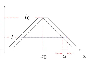
Figure 1. The truncated cone
Appendix
To prove Proposition 2.1, we observe that according to Theorems A and 2, the operator T =e±it√−∆Nsatisfies
(3.50) kTu0kL5((0,1)×Ω) .ku0k H
7 10
N (Ω)
.
Applying the previous inequality to ∆u0, and using theLp elliptic regularity result
(3.51) −∆u+u=f ∈L
p(Ω), ∂
nu|∂Ω= 0 ⇒u∈W2,p(Ω)∩WN1,p(Ω) and kukW2,p(Ω).kfkLp(Ω), 1< p <+∞
we get
(3.52) kTu0kL5((0,1);W2,5(Ω)∩W1,5
N (Ω)).ku0kH
27 10
N (Ω)
and consequently by (complex) interpolation between (3.50) and (3.52),
(3.53) kTu0k
L5((0,1);W103 ,5
N (Ω))
.ku0kH1
N(Ω);
finally, by Sobolev embedding
(3.54) kTu0kL5((0,1);L10(Ω)).ku0kH1
N(Ω).
To conclude, we simply observe that
u= cos(tp−∆N)u0+
sin(t√−∆N) √
−∆N u1
and 1/√−∆N is an isometry from L2(Ω) toHN1(Ω), providing the result. The usual T T⋆ argument and Christ-Kiselev Lemma [4] proves the following:
Proof. — We have
u(t,·) = cos(tp−∆N)u0+
sin(t√−∆N) √
−∆N
u1+ Z t
0
sin((t−s)√−∆N) √
−∆N
f(s,·)ds.
The contributions of (u0, u1) are easily dealt with, as previously. Let us focus on the
contribution of Z
t
0
ei(t−s)√−∆N
√ −∆N
f(s,·)ds.
Denote by T =eit√−∆N; interpolating between (3.50) and (3.52),
kTfk
L5((0,1);W2−7
Letu0 ∈L2. Then there exist v0∈HN2(Ω) such that
−∆v0=u0, ku0kL2 ∼ kv0kH2; as a consequence, fromTu0 = ∆Tv0,
kTu0k
L5((0,1);W−7
10,5(Ω)) .kTv0kL5((0,1);W2−7
10,5(Ω))∩WN1,5(Ω))
.kv0kH2
N(Ω)∼ ku0kL2(Ω).
By duality we deduce that the operatorT∗ defined by
T∗f = Z 1
0
e−is√−∆f(s,·)ds
is bounded from L54((0,1);W107,54(Ω)) to L2(Ω) (observe that W107,54(Ω) = W 7 10,54 N (Ω)); using (3.53) and boundedness of √−∆N−1 from L2 to HN1, we obtain
kT(p−∆N)−1T∗fk
L5((0,1);W103,5
N (Ω))∩L
∞
((0,1);H1
N(Ω))
.kfk
L54((0,1);W 7 10,54
N (Ω))
,
and
k∂tT(
p
−∆N)−1T∗fkL∞
((0,1);L2(Ω))≤Ckfk
L54((0,1);W 7 10,54
N (Ω))
.
But
T(p−∆N)−1T∗f(s,·) =
Z 1
0
ei(t−s)√−∆N
√ −∆N
f(s,·)ds
and an application of Christ-Kiselev lemma [4] allows to transfer this property to the operator
f 7→ Z t
0
ei(t−s)√−∆N
√ −∆N
f(s,·)ds.
References
[1] Ramona Anton. Strichartz inequalities for Lipschitz metrics on manifolds and nonlinear Schr¨odinger equation on domains, 2005. preprint,arXiv:math.AP/0512639.
[2] Nicolas Burq, Patrick G´erard, and Nikolay Tzvetkov. Strichartz inequalities and the nonlinear Schr¨odinger equation on compact manifolds. Amer. J. Math., 126(3):569–605, 2004.
[3] Nicolas Burq, Gilles Lebeau, and Fabrice Planchon. Global existence for energy critical waves in 3-D domains, 2006. preprint,arXiv:math.AP/0607631.
[4] Michael Christ and Alexander Kiselev. Maximal functions associated to filtrations.J. Funct. Anal., 179(2):409–425, 2001.
[5] Manoussos G. Grillakis. Regularity and asymptotic behaviour of the wave equation with a critical nonlinearity.Ann. of Math. (2), 132(3):485–509, 1990.
[6] Sergiu Klainerman and Matei Machedon. Remark on Strichartz-type inequalities. Internat. Math. Res. Notices, (5):201–220, 1996. With appendices by Jean Bourgain and Daniel Tataru. [7] Gilles Lebeau. Estimation de dispersion pour les ondes dans un convexe. In Journ´ees
“ ´Equations aux D´eriv´ees Partielles” (Evian, 2006). 2006.
[9] Jeffrey Rauch. I. The u5
Klein-Gordon equation. II. Anomalous singularities for semilinear wave equations. InNonlinear partial differential equations and their applications. Coll`ege de France Seminar, Vol. I (Paris, 1978/1979), volume 53 ofRes. Notes in Math., pages 335–364. Pitman, Boston, Mass., 1981.
[10] Jalal Shatah and Michael Struwe. Regularity results for nonlinear wave equations. Ann. of Math. (2), 138(3):503–518, 1993.
[11] Jalal Shatah and Michael Struwe. Well-posedness in the energy space for semilinear wave equations with critical growth. Internat. Math. Res. Notices, (7):303ff., approx. 7 pp. (elec-tronic), 1994.
[12] Hart F. Smith and Christopher D. Sogge. On the critical semilinear wave equation outside convex obstacles.J. Amer. Math. Soc., 8(4):879–916, 1995.
[13] Hart F. Smith and Christopher D. Sogge. On the Lp norm of spectral clusters for compact
manifolds with boundary, 2006. to appear, Acta Matematica,arXiv:math.AP/0605682. [14] Michael Struwe. Globally regular solutions to the u5
Klein-Gordon equation. Ann. Scuola Norm. Sup. Pisa Cl. Sci. (4), 15(3):495–513 (1989), 1988.
[15] Terence Tao. Local well-posedness of the Yang-Mills equation in the temporal gauge below the energy norm.J. Differential Equations, 189(2):366–382, 2003.
[16] Daniel Tataru. Strichartz estimates for second order hyperbolic operators with nonsmooth coefficients. III.J. Amer. Math. Soc., 15(2):419–442 (electronic), 2002.
[17] Daniel Tataru. On the regularity of boundary traces for the wave equation. Ann. Scuola Norm. Sup. Pisa Cl. Sci. (4), 26(1):185–206, 1998.
N. Burq, Universit´e Paris Sud, Math´ematiques, Bˆat 425, 91405 Orsay Cedex, France et Institut Universitaire de France • E-mail :[email protected]