Nonlinear Robust
H
∞
Static Output Feedback Controller Design for
Parameter Dependent Polynomial Systems: An Iterative Sum of
Squares Approach
Matthias Krug, Shakir Saat and Sing Kiong Nguang
Abstract— The design of a robust nonlinearH∞static output
feedback controller for parameter dependent polynomial sys-tems is a hard problem. This paper presents a computational relaxation in form of an iterative design approach. The pro-posed controller guarantees theL2-gain of the mapping from exogenous input noise to the controlled output is less than or equal to a prescribed value. The sufficient conditions for the existence of nonlinearH∞ static output feedback controller are
given in terms of solvability conditions of polynomial matrix inequalities, which are solved using sum of squares decompo-sition. Numerical examples are provided to demonstrate the validity of the applied methods.
I. INTRODUCTION
The problem of designing a nonlinear H∞ controller has
attracted considerable attention for more than three decades, see for instance [1], [2], [3], [4]. Generally speaking, the aim of anH∞ control problem is to design a controller such
that the resulting closed-loop control system is stable and a prescribed level of attenuation from the exogenous distur-bance input to the output inL2/l2-norm is fulfilled. There are
two common approaches available to address nonlinear H∞
control problems: One approach is based on the dissipativity theory [5] and theory of differential games [1]; The other is based on the nonlinear version of the classical bounded real lemma as developed in [6] and [7]. The underlying idea behind both approaches is the conversion of the nonlinearH∞
control problem into solvability conditions of the Hamilton-Jacobi equation (HJE). Unfortunately, this representation is hard to solve and it is generally very difficult to find a global solution.
A computational relaxation on the solvability conditions of the HJE has been presented in [8] by using a sum of squares (SOS) decompositions of polynomial terms. In detail, the relaxation uses Gram Matrix methods to efficiently transform the HJE into linear matrix inequalities (LMIs) [9]. This representation of the NP-hard problem can in turn be solved in polynomial time with semidefinite programming (SDP) [10], [11]. There exist several freely available toolboxes to formulate these problems in Matlab, for example SOS-TOOLS [12], YALMIP [13], CVX [14], and GloptiPoly [15]. Whereas SOSTOOLS is specifically designed to address polynomial nonnegativity problems, the latter toolboxes have further functionality, such as modules to solve the dual of the SOS problem, the moment problem.
M. Krug, S. Saat, and S.K. Nguang are with the Department of Electrical and Computer Engineering, The University of Auckland, 92019 Auckland, New [email protected]
In [16], [17], [18], [19], several approaches utilizing SOS decompositions to achieve nonlinear H∞ control are
presented. The systems discussed are represented in a state dependent linear-like form. In addition, the authors assumed that the control input matrix has some zero rows and the Lyapunov function only depends on states whose corre-sponding rows in control matrix are zeros, that is, the state dynamics are not directly affected by the control input. This assumption, however, leads to a conservative controller design.
The problem of static output feedback is stated as follows: given a system, find a static output feedback gain such that the closed loop system is stable. The static output formulation can be used to design a full order dynamic controller, but the converse is not true [20]. An iterative LMI (ILMI) procedure to compute the static output feedback gain for linear systems can be found in [21]. The result has been extended to nonlinear systems using a Takagi-Sugeno (TS) fuzzy model to approximate the system’s nonlinearities in [22]. Here, the ILMI methodology has been used to solve bilinear matrix inequalities. Further, in [23], the ILMI method was used to obtain a nonlinear H∞ static output
controller for TS fuzzy models. The authors assumed that the premises variables are bounded. In general, however, the premises variables are related to the state variables and thus this assumption implies that the state variables also have to be bounded. This is the main drawback of the TS fuzzy model approach. Furthermore, TS fuzzy models are restricted to quadratic Lyapunov functions, which adds conservatism to the design process.
To the best of authors’ knowledge, there is no general result on nonlinear static output feedback design for polyno-mial systems. Even though [24] addressed this problem, it uses the same conservative assumptions as in [19] where control matrix and Lyapunov function have to be of a particular form and require certain parameters to be equal to zero. By making this assumption, it is capable of avoiding non-convex terms in the static output feedback design, but results in a more conservative design. The main contributions of this paper can be summarized as follows:
• The proposed controller design avoids rational static output feedback controllers due to the inversion of the Lyapunov function.
• The Lyapunov function does not require to be function of states whose corresponding rows in control matrix are zeroes.
2011 50th IEEE Conference on Decision and Control and European Control Conference (CDC-ECC)
• The Lyapunov function is not restricted to be in quadratic form, but can take higher order even degree forms.
The remainder of this paper is organized as follows: Section II provides the preliminaries and notations used throughout the remainder of the paper. The main results are highlighted in section III. The validity of our proposed approach is illustrated through examples in Section IV. Finally, conclusions are drawn in Section V.
II. PRELIMINARIES ANDNOTATIONS
In this section, we introduce the notation that will be used in the remainder of the paper. Furthermore, we provide a brief review on SOS decomposition. For a more elaborate description of SOS decompositions see for example [8].
A. Notations
Let R be the set of real numbers and Rn be the n-dimensional real space. Furthermore, let In represent the
identity matrix of sizen×n.Q"0(Q#0)is used to express the positive (semi)definiteness of (the square) matrixQ.
When talking about partial derivatives of a Lyapunov functionV(x)innvariables, we denote∂V∂(xx) as a row vector, i.e. ∂V∂(xx)=!∂V∂x(x)
1 ,
∂V(x)
∂x2 , . . . ,
∂V(x)
∂xn
" .
We use ℜm to describe the set of all polynomials in m
variables with real coefficients. A polynomial vector field is then defined as f :Rm→Rm,f(x) = [f
1(x), . . . ,fm(x)]T,
where each fi∈ℜm.
A (∗) is used to represent transposed symmetric matrix entries.
B. SOS Decomposition
Definition 2.1: A multivariate polynomial f(x), forx∈ℜn
is a sum of squares if there exist polynomials fi(x),i=1, ...,n
such that
f(x) = n
∑
i=1
fi2(x). (1)
It is apparent from definition 2.1 that the set of SOS polynomials in n variables is a convex cone, and it is also true (but not obvious) that this convex cone is proper [25]. If a decomposition of f(x)in the above form can be obtained, it is clear that f(x)≥0,∀x∈Rn. The converse, however, is generally not true.
The problem of finding the right hand side of (1) can be formulated in terms of the existence of a positive semidefinite matrixQsuch that the following proposition holds:
Proposition 2.1: [8] Let f(x)be a polynomial in x∈ℜn
of degree 2d. LetZ(x)be a column vector whose entries are all monomials inxwith degree≤d. Then, f(x)is said to be SOS if and only if there exists a positive semidefinite matrix
Qsuch that
f(x) =Z(x)TQZ(x). (2) In general, determining the non-negativity of f(x) for
deg(f)≥4 is classified as a NP-hard problem [26], [27]. However, using Proposition 2.1 to formulate nonnegativity conditions of a polynomial provides a relaxation that is computational traceable.
III. MAINRESULTS
In this section, we start with the derivation of an H∞
controller. The results are subsequently extended to the robust control synthesis.
A. H∞Static Output Feedback Control
Consider the following dynamic model of a polynomial system:
˙
x=A(x) +Bu(x)u+Bω(x)ω
y=Cy(x) +Dy(x)u
z=Cz(x) +Dz(x)u
(3)
where ω ∈Rp is the disturbance and z is the output to be regulated. A(x),Cy(x),Cz(x) are polynomial vectors and
Bu(x),Bω(x),Dy(x),Dz(x)are polynomial matrices of
appro-priate dimensions. The H∞ static output feedback control
problem can be described as follows. Given a system (3), find a controller of the from
u=K(y) (4) such that the closed-loop system is asymptotically stable and theL2gain of the mapping of the energy from the exogenous
input disturbance to the regulated output is less than or equal to a prescribedH∞ performance γ>0, i.e.
' ∞
0
zTzdt≤γ2' ∞ 0
ωTωdt. (5)
Proposition 3.1: The system (3) without noise, i.e. ω= 0 is stabilizable via static output feedback if there exists a nonlinear functionV(x) and a nonlinear matrix K(y) such that the following conditions hold
V(x)>0 x*=0
V(x) =0 x=0 (
, (6)
and
∂V(x)
∂x A(x)−
1 4
∂V(x)
∂x Bu(x)B
T u(x)
∂VT(x)
∂x +
Θ(x,y)Θ(x,y)T<0, (7)
where Θ(x,y)is defined as
Θ(x,y) =
) 1 2
∂V(x)
∂x Bu(x) +K
T(y) *
. (8)
Proof:omitted due to space limitations.
Theorem 3.1: The system (3) is stabilizable with a pre-scribedH∞performance γ>0 via static output feedback of
form (4) if there exist a nonlinear function V(x) satisfying (6) and a nonlinear matrix K(y) such that for ∀x*=0 the following holds
∂V(x)
∂x A(x)−
1 4
∂V(x)
∂x Bu(x)B
T u(x)
∂VT(x)
∂x
+ )
1 2
∂V(x)
∂x Bω(x)
* 1
γ2 )
1 2
∂V(x)
∂x Bω(x)
*T
+ )
1 2
∂V(x)
∂x Bu(x) +K
T(y) * )
1 2
∂V(x)
∂x Bu(x) +K
T(y) *T
If conditions (6) and (9) hold, the closed-loop system is asymptotically stable.
Proof: omitted due to space limitations.
The advantages of formulating the conditions of the static output feedback problem with prescribedH∞performance γ
in the form of Theorem 3.1 are twofold: 1) a more suitable form for numerical procedures can be developed, and 2) the static output feedback controller is no longer assumed to be a directly dependent function of the Lyapunov function. It is, however, not possible to directly implement (9) as a state-depended LMI due to the non-convex negative term −14∂V∂(xx)Bu(x)BTu(x)
∂VT(x)
∂x . This is addressed by introducing
the nonlinear design vector ε(x) of appropriate dimension. Using +ε(x)−∂V∂(xx),Bu(x)BTu(x) arrive at the following theorem.
Theorem 3.2: The system (3) is stabilizable by means of static output feedback (4) with a prescribed H∞ norm γ if there exists a nonlinear function V(x) satisfying (6), nonlinear matrix K(y), and nonlinear vector ε(x)such that the following condition hold
∂V(x)
Proof: omitted due to space limitations.
To relax the problem (11) computationally, we introduce the term αV(x),α∈R on the right hand side of (11), and note that α <0 implies that a feasible solution has been found. We arrive at the following proposition:
Proposition 3.2: The system (3) is stabilizable by means of static output feedback (4) withH∞normγif there exists a
nonlinear functionV(x)that satisfies (6), a nonlinear vector
ε(x), and a nonlinear matrix K(y)such that∀x*=0
One can readily verify Proposition 3.2 by applying Schur complement to Theorem 3.2.
B. Robust Stability Synthesis
The results presented in the previous section assume that all system parameters are known exactly. In this section, we investigate how the algorithm can be extended to systems in which the parameters are not exactly known.
Consider the following system
˙
∈Rqis the vector of constant uncertainty and satisfies
We further define the following parameter dependent Lya-punov function
With the results from the previous section, we can directly propose the main result for robustH∞static output feedback
control problem.
Theorem 3.3: Given SOS polynomial functionsλ1(x)>0
andλ2(x)>0 forx*=0, the system (14) with static output
feedback controller (4) and H∞ performance γ is stable if
Vi(x)satisfying (6), a polynomial vectorε(x) =∑qi=1εi(x)θi,
and a polynomial matrixK(y)such that forx=* 0,i=1, . . . ,q:
Vi(x)−λ1(x) is a SOS, (18) −vT6
Mαi(x,y) +λ2(x)I7v is a SOS. (19)
where vis of appropriate dimensions.
This theorem follows directly as a superposition of several systems of the form (3) with (4) for a common K(y) and Proposition 3.2.
The conditions given in Proposition 3.2 are presented in form of state depended bilinear matrix inequalities (BMIs). To solve (12) directly is, however, computationally hard and would require to solve an infinite set of state depen-dent BMIs. Further, the term −12ε(x)Bu(x)BTu(x)
∂VT(x)
∂x +
1
4ε(x)Bu(x)BTu(x)εT(x) makes (12) non-convex, hence the
inequality cannot be solved directly by SOS decomposition and SDP. If, however, the auxiliary polynomial vector ε(x) is fixed, (12) becomes convex and can be solved efficiently. Unfortunately, fixingε(x)generally does not yield a feasible solution. Therefore, we propose the following iterative SOS (ISOS) procedure as an iterative search for Vi(x),K(y),
auxiliary variableεi(x), and parameter α.
Iterative Algorithm of Sum of Squares (ISOS)
Step 1: Linearize each system from (14) with (15) and set
ω =0. Use the static output feedback approach described in [21] to find a solution to the linearized problems without disturbance. Set t =1,εi
1(x) =
xTPi,i=1, . . . ,q.
Step 2: Solve the following SOS optimization problem in
Vi
t(x) and Kt(y) with fixed auxiliary polynomial
vectorsεi t(x):
Minimize αt
Subject toVti(x) +λ1(x), is a SOS, −vT6
Mαi(x,y) +λ2(x)I7v, is a SOS,
fori=1, . . . ,q,
where vis of appropriate dimensions.
If αt<0, thenV(x) =∑qi=1Vti(x)θi and Kt(y)
rep-resent a feasible solution. Terminate the algorithm. Step 3: Set t =t+1 and solve the following SOS opti-mization problem in Vti(x) and Kt(y) with αt =
αt−1 determined in Step 2 and noting the SOS
decomposition of Vti(x) =Z(x)TQi
tZ(x) with Z(x)
being a vector of monomials in x up to some predefined degree:
Minimize
q
∑
i=1
trace(Qit)
Subject toVti(x) +λ1(x), is a SOS, −vT6Mαi(x,y) +λ2(x)I
7
v, is a SOS, fori=1, . . . ,q.
Step 4: Solve the following feasibility problem with v2∈
Rn+1 and a predefined positive tolerance function
δ(x)>0,x*=0:
vT2
8 δ(x) ( ∗) +
εi t(x)−
∂Vti(x)
∂x
,T 1
9
v2, is a SOS,
fori=1, . . . ,q.
If the problem is feasible go to Step 5. Else, set
t=t+1 andεi t(x) =
∂Vi
t−1(x)
∂x ,i=1, . . . ,qdetermined
in Step 3 and go to Step 2.
Step 5: The system (14) may not be stabilizable with H∞
performance γ by static output feedback (4). Ter-minate the algorithm.
Remark 3.1:
• Step 1 is used to find an appropriate value of ε1(x)to
use as an initial guess to fulfill (12).
• The optimization problem in Step 2 is a generalized eigenvalue minimization problem and guarantees the progressive reduction ofαi. Meanwhile, Step 3 ensures
convergence of the algorithm.
• The iterative algorithm increases the iteration variablet twice per iteration. This is done to avoid confusion with the indices used.
IV. NUMERICALEXAMPLE
In this section, we will provide two design examples to demonstrate the validity of the proposed static output feedback controller withH∞ performance γ.
Example 1: Lorenz Chaotic System.The dynamics of the
Lorenz Chaotic System can be described as follows
˙
x=
−ax1+ax2
cx1−x2−x1x3
x1x2−bx3
+
1 0 0
u. (20)
The system exhibits chaotic behavior fora=10,b=8/3,c= 28. xi are the system states and u the control input. We
assume z=y=x2. Furthermore, we assume that there is
a disturbance present for x3 and that the system dynamics
are not exactly known an are somewhere between the two vertexes
˙
x1=
−ax1+ax2
cx1−x2+x1x3
x1x2−bx3
+
1 0 0
u+
0 0 1
ω
±0.1
−ax1+ax2
cx1 −bx3
+
1 0 0
u
(21)
We selectλ1(x) =λ2(x) =δ(x) =0.016x21+x22+x23 7
. Using the described ISOS procedure, we initially choose the degree of the Lyapunov function to be 2 and allow the polynomial static controller to be of the formK(y) =k1y+k2y2, but no
feasible solution could be obtained. Increasing the degree to 4, however, yields a feasible solution with k2≈0. Fixing
K(y) to be a linear static output feedback controller, the following controller withH∞ normγ=1.567 was obtained
after 4 iterations:
0 0.2 0.4 0.6 0.8 1 1.2 1.4 1.6 1.8 2
−20
0 20
Time (s)
x1
(t)
0 0.2 0.4 0.6 0.8 1 1.2 1.4 1.6 1.8 2 0
20 40
Time (s)
x2
(t)
0 0.2 0.4 0.6 0.8 1 1.2 1.4 1.6 1.8 2
−20 −10
0
Time (s)
x3
(t)
Fig. 1. Example 1: Lorenz Chaotic System
with Lyapunov functions
V1(x) =1.7697x41+0.2174x13x2+2.6537x21x22 +0.9376x21x23−1.7438x21x3+48.2846x21 +0.1478x1x2x3+37.3706x1x2+0.7284x42 +0.1368x22x23+0.6956x22x3+31.4986x22 +0.0078x43−0.0168x33+2.2961x32,
(23)
V2(x) =1.9058x41+0.2234x31x2+1.9775x21x22 +0.5366x21x23−2.2914x21x3+71.2832x21 +0.0136x1x2x3+40.411x1x2+0.3359x42 +0.0859x22x23+0.3574x22x3+28.165x22 +0.0068x43−0.0026x33+2.0306x23.
(24)
The simulation results for both vertexes as well as the nominal plant for the initial conditions x0 = 3
20, −10, −204T have been plotted in Figure 1.
Example 2: Polynomial System.Consider the polynomial
system from [24]:
A1(x) = >
−x1+x21−32x 3 1−34x1x
2
2+14x2−x 2
1x2−12x32
0
? ,
Bu1(x) = >
0 1 ?
, Bω1(x) = >
1 0 ?
,
Cy1(x) =x1−x2, Dy1(x) =0, Cz1(x) =0, Dz1(x) =1,
A2(x) = >
−x1+x21−32x 3
1+14x2−x 2 1x2
0
? ,
Bu2(x) = >
0 1.2
?
, Bω2(x) = >
1.5 0
?
, Cy2(x) =x1−x2,
Dy2(x) =0, Cz2(x) =0, Dz2(x) =1. (25)
The system is characterized by one pure integrator and therefore the the open-loop system is clearly not stable. We selectλ1(x) =λ2(x) =δ(x) =0.01
6
x21+x22+x237, allowK(y) to be of the form K(y) =k1y+k2y2+k3y3 and look for a
Lyapunov function of degree 4. The algorithm terminates with a feasible solution and very small coefficients k2 and
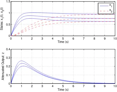
0 1 2 3 4 5 6 7 8 9 10 0
0.5 1 1.5
Time (s)
States: x
1
(t), x
2
(t)
x
1
x
2
0 1 2 3 4 5 6 7 8 9 10 0
0.1 0.2 0.3 0.4
Time (s)
Attenuated Output: z
Fig. 2. Example 2: Polynomial System. Constant disturbance
k3. Thus, we decide to investigate whether a feasible solution
can be obtained while limiting the controller to be of linear nature. After 6 iterations the algorithm terminates and the followingH∞static output feedback controllerγ=1.514 has
been obtained
K(y) =0.380y. (26) The corresponding Lyapunov functions are as follows
V1=0.1083x41+0.0088x31x2+0.0564x31 +0.0484x21x22+0.0852x21x2+0.2817x21 +0.1796x1x32−0.0602x1x22−0.1084x1x2 +0.1219x42−0.069x32+0.621x22,
(27)
V2=0.0834x41+0.0864x31x2+0.0346x31 +0.0195x21x22+0.0584x21x2+0.2806x21 +0.0072x1x32−0.0122x1x22−0.156x1x2 +0.0484x42−0.0426x32+0.5302x22.
(28)
The simulation result are shown in two steps to allow a comparison with the results presented in [24]. Figure 2 shows the system response of the system from a steady state to a constant disturbanceω=1 for the two vertexes and a system that lies in between. It can be seen that our controller is stabilizing the system and the attenuated output is always less than 0.3. Comparing our results to the ones presented in [24], one can see that the disturbance has a smaller influence on the attenuated output. This result is to be expected, as our γ is smaller than their result of γ=1.8071. Since our controller has a smaller gain compared to the one in [24], our states settle to steady state that is further from the origin.
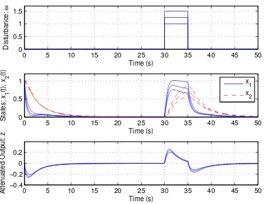
In Fig. 3, we show the system response for the vertexes and a system in between the two from the initial conditions
x0=31, 14 T
. The controller proposed in [24] as well as ours show similar system trajectories. It should be noted, however, that due to the lower γ-value for our H∞ static
0 5 10 15 20 25 30 35 40 45 50 0
0.5 1 1.5
Time (s)
Disturbance:
ω
0 5 10 15 20 25 30 35 40 45 50 0
0.5 1
Time (s)
States: x
1
(t), x
2
(t)
x
1
x2
0 5 10 15 20 25 30 35 40 45 50
−0.4 −0.2
0 0.2
Time (s)
Attenuated Output: z
Fig. 3. Example 2: Polynomial System. Closed-loop behavior
V. CONCLUSION
We have introduced and discussed the concept of a robust
H∞ static output feedback control design for polynomial
systems. In detail, we have introduced an iterative algorithm to solve the state-dependent BMIs efficiently. By introduc-ing a less restrictive choice of the form of the Lyapunov function by allowing higher degree polynomials, we were able to formulate a less conservative approach. Furthermore, removing the direct coupling of the Lyapunov function and the controller matrix in the problem formulation facilitates the design of linear controllers for higher order polynomial systems. Additionally, the simulation results indicate that the result is less conservative than previous approaches.
VI. ACKNOWLEDGMENTS
The authors gratefully acknowledge the support in part by The University of Auckland, Technical University of Malaysia Malacca (UTeM), and Government of Malaysia Scholarship.
REFERENCES
[1] J. Ball and J. Helton, “H∞ control for nonlinear plants: connections
with differential games,” inConference on Decision and Control, 1989, pp. 956–962.
[2] T. Bas¸ar and G. J. Olsder, Dynamic noncooperative game theory. London; New York: Academic Press, 1995.
[3] A. van der Schaft, “L2-gain analysis of nonlinear systems and
non-linear state-feedback H∞ control,”IEEE Transactions on Automatic
Control, vol. 37, no. 6, pp. 770–784, 1992.
[4] A. Isidori and A. Astolfi, “Disturbance attenuation andH∞-control via
measurement feedback in nonlinear systems,”IEEE Transactions on Automatic Control, vol. 37, no. 9, pp. 1283–1293, 1992.
[5] T. Bas¸ar, “Optimum performance levels for minimax filters, predictors and smoothers,”Systems & Control Letters, vol. 16, no. 5, pp. 309– 317, 1991.
[6] D. J. Hill and P. J. Moylan, “Dissipative dynamical systems: Basic input-output and state properties,” Journal of the Franklin Institute, vol. 309, no. 5, pp. 327–357, 1980.
[7] J. C. Willems, “Dissipative dynamical systems part i: General theory,” Archive for Rational Mechanics and Analysis, vol. 45, pp. 321–351, 1972.
[8] P. A. Parrilo, “Structured semidefinite programs and semialgebraic geometry methods in robustness and optimization,” Ph.D. Thesis, California Institute of Technology, May 2000.
[9] V. Powers and T. W¨ormann, “An algorithm for sums of squares of real polynomials,”Journal of Pure and Applied Algebra, vol. 127, no. 1, pp. 99–104, 1998.
[10] L. Vandenberghe and S. P. Boyd, “Semidefinite programming,”SIAM Review, vol. 38, no. 1, pp. 49–95, 1996.
[11] S. P. Boyd, L. E. Ghaoui, E. Feron, and V. Balakrishnan,Linear matrix inequalities in system and control theory. Philadelphia: SIAM, 1994. [12] S. Prajna, A. Papachristodoulou, and P. A. Parrilo, “Introducing SOSTOOLS: a general purpose sum of squares programming solver,” inConference on Decision and Control, vol. 1, 2002, pp. 741–746. [13] J. L¨ofberg, “YALMIP: a toolbox for modeling and optimization
in Matlab,” in IEEE International Symposium on Computer Aided Control Systems Design, 2004, pp. 284–289.
[14] M. Grant and S. Boyd, “Graph implementations for nonsmooth convex programs,” inRecent Advances in Learning and Control, ser. Lecture Notes in Control and Information Sciences, V. Blondel, S. Boyd, and H. Kimura, Eds. Springer-Verlag Limited, 2008, pp. 95–110. [15] D. Henrion, J.-B. Lasserre, and J. L¨ofberg, “GloptiPoly 3: moments,
optimization and semidefinite programming,” Optimization Methods and Software, vol. 24, no. 4, pp. 761–779, 2009.
[16] S. Prajna, A. Papachristodoulou, and F. Wu, “Nonlinear control syn-thesis by sum of squares optimization: a Lyapunov-based approach,” inAsian Control Conference, vol. 1, 2004, pp. 157–165.
[17] A. Papachristodoulou and S. Prajna, “On the construction of Lyapunov functions using the sum of squares decomposition,” inConference on Decision and Control, vol. 3, 2002, pp. 3482–3487.
[18] H.-J. Ma and G.-H. Yang, “Fault-tolerant control synthesis for a class of nonlinear systems: Sum of squares optimization approach,” International Journal of Robust and Nonlinear Control, vol. 19, no. 5, pp. 591–610, 2009.
[19] D. Zhao and J.-L. Wang, “An improvedH∞ synthesis for
parameter-dependent polynomial nonlinear systems using SOS programming,” in American Control Conference, 2009, pp. 796–801.
[20] V. Syrmos, C. Abdallah, P. Dorato, and K. Grigoriadis, “Static output feedback - a survey,”Automatica, vol. 33, no. 2, pp. 125–137, 1997. [21] Y.-Y. Cao, J. Lam, and Y.-X. Sun, “Static output feedback stabilization: An ILMI approach,”Automatica, vol. 34, no. 12, pp. 1641–1645, 1998. [22] D. Huang and S. K. Nguang, “Static output feedback controller design for fuzzy systems: An ILMI approach,”Journal of Information Sciences, vol. 177, no. 14, pp. 3005–3015, 2007.
[23] D. Huang and S. K. Nguang, “Robust H∞ static output feedback
control of fuzzy systems: An ILMI approach,”IEEE Transactions on Systems, Man, and Cybernetics, Part B: Cybernetics, vol. 36, no. 1, pp. 216–222, 2006.
[24] D. Zhao and J.-L. Wang, “Robust static output feedback design for polynomial nonlinear systems,”International Journal of Robust and Nonlinear Control, vol. 20, no. 14, pp. 1637–1654, 2010.
[25] H. Hindi, “A tutorial on convex optimization,” inAmerican Control Conference, vol. 4, 2004, pp. 3252–3265.
[26] A. Papachristodoulou and S. Prajna, “A tutorial on sum of squares techniques for systems analysis,” in American Control Conference, vol. 4, 2005, pp. 2686–2700.