International Journal of Advanced Robotic Systems
Thruster Modelling
for Underwater Vehicle Using
System Identification Method
Regular Paper
Mohd Shahrieel Mohd Aras
1,*, Shahrum Shah Abdullah
2,
Azhan Ab. Rahman
1and Muhammad Azhar Abd Aziz
21 Department of Mechatronics, Faculty of Electrical Engineering,
Universiti Teknikal Malaysia Melaka, Hang Tuah Jaya, Durian Tunggal, Melaka, Malaysia 2 Department of Electric and Electronics, Malaysia-Japan International Institute of Technology, Universiti Teknologi Malaysia, International Campus Jalan Semarak, Kuala Lumpur, Malaysia * Corresponding author E-mail: [email protected]
Received 11 May 2012; Accepted 22 Mar 2013
DOI: 10.5772/56432
© 2013 Aras et al.; licensee InTech. This is an open access article distributed under the terms of the Creative Commons Attribution License (http://creativecommons.org/licenses/by/3.0), which permits unrestricted use, distribution, and reproduction in any medium, provided the original work is properly cited.
Abstract This paper describes a study of thruster
modelling for a remotely operated underwater vehicle
(ROV) by system identification using Microbox
2000/2000C. Microbox 2000/2000C is an XPC target
machine device to interface between an ROV thruster
with the MATLAB 2009 software. In this project, a model
of the thruster will be developed first so that the system
identification toolbox in MATLAB can be used. This
project also presents a comparison of mathematical and
empirical modelling. The experiments were carried out
by using a mini compressor as a dummy depth pressure
applied to a pressure sensor. The thruster model will
thrust and submerge until it reaches a set point and
maintain the set point depth. The depth was based on
pressure sensor measurement. A conventional
proportional controller was used in this project and the
results gathered justified its selection.
Keywords System identification (SI), Pressure Sensor,
Remotely Operated Underwater Vehicle, Microbox
2000/2000C
1. Introduction
A thruster is an electromechanical device equipped with
a motor and propeller that generates thrust to push an
Underwater Vehicle. Thruster control and modelling are
important parts of underwater vehicle control and
simulation. This is because it is the lowest control loop of
the system; hence, the system would benefit from
accurate and practical modelling of the thrusters [1]. In
underwater vehicles such as ROV and AUV, thrusters are
generally propellers driven by electrical DC motors.
Therefore, thrust force is simultaneously affected by
motor model, propeller design, and hydrodynamic effects [2, 3]. There are also many other factors to consider which
make the modelling procedure difficult. To resolve the
difficulties, this paper will describe thruster models that
have been proposed using Microbox 2000/2000C.
Microbox 2000/2000C is a solution for prototyping,
testing and developing real‐times system using standard
PC hardware for running real‐time applications, as shown in Figure 1. Microbox 2000/2000C acts as a microcontroller, and is also called the “XPC target machine”. Microbox 2000/2000C is a rugged, high‐ performance x86‐based industrial PC with no moving parts inside. It supports all standard PC peripherals such as video, mouse, and keyboard. For engineers who have real‐time analysis and control‐system testing needs, Microbox 2000/2000C offers an excellent mix of performance, compactness, sturdiness, and I/O expandability [4]. Microbox 2000/2000C is used integrated with MATLAB/Simulink and related control modules. It can run real‐time modelling and simulation of control systems, rapid prototyping, and hardware‐in‐the‐loop testing. And These tasks do not need any manual code generation or complicated debugging processes. The result benefits users in terms of cost and time saving, and makes the control system design and testing easy to accomplish, also allowing flexibility when dealing with complex control systems [5].
Figure 1. Microbox 2000/2000C
This paper is organized as follows. Section 2 gives a brief introduction to system identification and the mathematical modelling of thrusters. Section 3 presents the fabrication process of a pressure sensor including testing and interfacing with Microbox. Section 4 describes system identification simulation results using the derived thruster model and algorithms. Section 5 illustrates the field testing results. Section 6 presents final remarks.
2. Theoretical issues
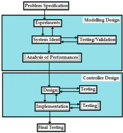
This section will describe the theoretical aspects of the project. The methodology will also be described, in terms of system identification, as shown in Figure 2. Finally, the general equation for thrusters will be summarized. The derivation of the thruster model was based on the experiment presented in [6]. This project involves a varied model generated by system identification that can be used in modelling the Underwater Vehicle. This model will be integrated with ROV for depth control. The depth measured was based on pressure sensor design.
Figure 2. Flow chart of design and modelling of thruster
2.1 System Identification
For system identification, the development of the Underwater Vehicle will be considered first and will be referred to as platform development. The methodology in this project is shown in Figure 3.
Figure 3. Methodology of project
The first stage is establishing the design parameters. The dynamic motion equation must first be familiarized. In this project, the Mathematical Model of Vertical Movement (depth movement) is studied. A combination of rigid body motion and fluid mechanics principles, an underwater robot motion model can be derived from the dynamics equation of an underwater vehicle [7]. The dynamics of a 6‐degree‐of‐freedom underwater vehicle can be described thus:
��� � ����� � ����� � ���� � ����� (1)
where
M is the 6 x 6 inertia matrix including hydrodynamic added mass;
g(η) is the vector of restoring forces and moments;
B(v) is the 6 x 3 control matrix.
� � ���� is the mass matrix that includes rigid body and
added mass, and satisfies M = MT > O and �� = 0 ; C(ν) � ����
is the matrix of Coriolis and centrifugal terms including added mass, and satisfies C(ν) = ‐C(ν)T ; D(ν) � ���� is the
matrix of friction and hydrodynamic damping terms;
g(η) � �� is the vector of gravitational and buoyancy
generalized forces; η� �� is the vector of Euler angles; ν� �� is the vector of vehicle velocities in its 6 DOF, relative to the fluid and in a body‐fixed reference frame; and τ� �� is the driver vector considering the vehicle’s thruster positions.
After identifying the design parameters, the next stage is platform development. In this stage, the prototype underwater vehicle will be developed. System identification will take place once the platform is ready to be run. MATLAB System Identification Toolbox will be used. Some theory for SI must be cleared so that the model obtained is acceptable. The model obtained from System Identification will then be verified.
2.2 Thruster model
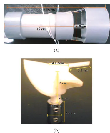
The thruster dynamics are still very much neglected and the oscillations are usually ignored or tolerated, based on the experiment presented in [6]. The thruster design in this project was developed by UTeRG, as shown in Figure 4. This paper will derive the thruster model for the under‐ actuated condition from the propeller’s hydrodynamics and the motor’s electromechanical properties. A hydrodynamic propeller model can be derived from basic Newtonian fluid mechanics theory and is shown in [6]:
T = KT0ω + KTω 2 (Nm) (2)
where
T = thruster output thrust;
ω = the propeller rotational speed;
KT0 , KT = lump parameter of various constants.
The electromechanical model of a motor that relates the applied voltage, V, to the thruster output T
V = RmI + Lmİ + KEω (3) T = KmI (4)
I = the current flowing in the motor armature Rm = motor resistance
Lm = motor inductance KE = motor back EMF constant Km = modified motor constant.
The simulated result of transient response does not match with the observed oscillatory thrust values measured with the force sensor. This may originate in the experimental
set‐up in [6]. In this experiment, thruster transient can be tolerated and thus can be ignored [6]. Only the steady state components of the thruster model have been considered. Based on Equation 2 and Equation 3:
T = KTω 2 (5) V = RmI + KEω (6)
Equation 4 substituted into Equation 5 and Equation 6: I = ���
T = KTω 2 ω = ����
� �
V = ������� � ������� � (7)
(a)
(b)
Figure 4. Thruster design by UTeRG
(a)
(b)
Figure 5 shows the parameter of thruster design in terms of body, propeller and coupling. Table 1 shows the motor parameters. These parameters will be used to obtain the DC motor thruster model.
Physical quantity Symbol Numerical value Armature inductance La 0.004690891710127 H Back‐emf constant Kb 0.018259462399963 Vs/rad Armature resistance Ra 2.560403088365053 Ω Torque motor Tf 0.000331085454438 Nm Total load inertia Jm 0.000072019412423 kgm 2 Viscous‐friction coefficient Cm/B 0.000091357863014
Nms/rad
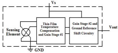
In the MPX4250A/MPXA4250A series, a Manifold Absolute Pressure (MAP) sensor for engine control is designed to sense absolute air pressure within the intake of the manifold. This measurement can be used to measure depth. The pressure sensor used for underwater depth measurement by using MPX4250AP CASE 867B‐04 is from Farnell, as shown in Figure 6. Only pin numbers 1, 2, and 3 will be used; the rest will not be connected. Figure 7 shows the fully integrated pressure sensor schematic. Based on the schematic, the pressure sensor has a sensing element, thin film temperature compensation, gain stage 1 cascaded with gain stage 2, and ground reference shift circuitry Figure 7. Fully Integrated Pressure Sensor Schematic
Figure 8 shows the recommended decoupling circuit for outside of the specified pressure range. The measurement unit will be in kPa. From the datasheet, the range of
Figure 8. Recommended Power Supply Decoupling and Output Filtering
(Temperature range from 0 to 85 o C)
Characteristic Symbol Value Units Supply Voltage Vs 5.1 VDC
Table 2. Operating characteristics [8]
3. Simulation
3.1 Thrust Control using Matlab/Simulink
Simulation using MATLAB/SIMULINK for propeller thrust control is shown in Figure 10. This propeller thrust control uses the conventional PID controller. Thruster design is based on the first‐order motor dynamic model. At the first simulation, there are no disturbances or faults in the system. The output of the speed control system is the thrust Ta and torque Qa, respectively.
Figure 10. Thrust control
Figure 11. Speed Control block diagram
The best gain for a PID controller such as Kp, Ki and Kd is equal to 5, 15, and 0, respectively Only the PI controller is actually sufficient for this system. When designing a PID controller for a given system, such as for the speed control as shown in Figure 11, the methods shown below are followed to obtain a desired response. Designers should try to keep the controller as simple as possible, but offering good performance [9, 10].
1. Kp: Proportional Gain ‐ Larger Kp typically means faster response since the larger the error, the larger the proportional term compensation. An excessively large proportional gain will lead to process instability and oscillation.
2. Ki: Integral Gain ‐ Larger Ki implies steady state errors are eliminated quicker. The trade‐off is larger overshoot: any negative error integrated during transient response must be integrated away by positive error before we reach steady state.
3. Kd: Derivative Gain ‐ Larger Kd decreases overshoot, but slow down transient response and may lead to instability due to signal noise amplification in the differentiation of the error.
Table 3 summarizes the effect of increasing the values of every gain Kp, Ki and Kd. In MATLAB tuning can be carried out automatically, meaning there is no need to tune every value of gain by trial and error.
Table 3. Effect of increasing Kp, Ki and Kd parameters in closed‐ loop system [11].
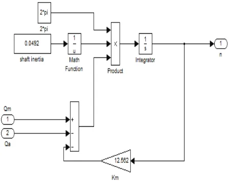
Figures 12 to 16 are block diagrams of a subsystem speed control system. Water density is set at 1024 kg/m³. Figure 17 and Figure 18 show the system response for thrust and torque generated. The system response for thrust showed the best response.
Figure 12. Reference thruster block diagram
Figure 13. First order motor dynamic model block diagram
Figure 15. Propeller load torque
Figure 16. Propeller thruster
Figure 17. System response
(a)
(b)
Figure 18. Torque response4. Results
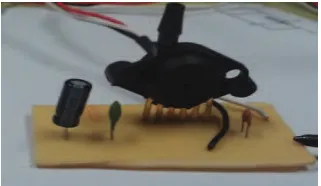
4.1 PCB Design for Depth Sensor
The next step is the PCB design process. PCB design for the pressure sensor consists of four important stages. Considerable care is required in the fabrication process since the design process is very sensitive to the tolerance in the dimension. The first stage is to prepare the master layout, followed by creating the photo‐resist pattern, etching and soldering.
Figure 19. Complete circuit
The complete circuit for the pressure sensor can be seen in Figure 19. The continuity is checked using a multimeter to ensure the complete flow of signal in the designed circuit. The pressure sensor is now ready to measure the water depth.
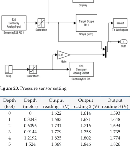
4.2 Testing Depth Sensor System using Microbox
The supply of the pressure sensor is constant at 5V from
the Microbox driver. The experiment for pressure sensors
uses three 1.5V batteries in series, equivalent to 4.5V. For
the initial value the display showed 1.848V, as shown in
Figure 20. To test the working of the pressure sensor, the test is set with a 41 cm level of water in a bucket. The
reading showed increasing pressure. This will then be
compared with the experiment in the pool. Table 4 shows
the results of the pressure sensor experiment. When the
depth is 41 cm the value on the pressure sensor is equal to 1.912V equivalent ± 40 cm.
Figure 20. Pressure sensor setting
Depth
(feet)
Depth
(meter)
Output
reading 1 (V)
Output
reading 2 (V)
Output
reading 3 (V)
0 0 1.622 1.614 1.593
1 0.3048 1.683 1.671 1.648
2 0.6096 1.731 1.716 1.694
3 0.9144 1.779 1.758 1.735
4 1.2192 1.825 1.802 1.774
5 1.524 1.869 1.846 1.826
6 1.8288 1.922 1.896 1.87
7 2.1336 1.973 1.944 1.886
8 2.4384 2.024 1.994 1.938
9 2.7432 2.054 2.03 1.983
10 3.048 2.122 2.085 2.032
11 3.3528 2.168 2.156 2.097
12 3.6576 2.223 2.207 2.174
Table 4. The results of the pressure sensor experiment
Figure 21. The results in Table 4 plotted onto a graph
Figure 21 shows a graph with the three readings from the
experiments in the pool. Comparison between datasheet
and experiment shows they are almost the same. So, this
pressure sensor can be said to be suitable to be applied on
an underwater vehicle.
4.3 Mini‐compressor as pressure depth
A mini‐compressor will be used to produce air pressure
for the pressure sensor to set the water depth as shown in
Figure 22. This compressor can supply up to 1 horse
power (1hp equal to 746 watt).
Specification Numerical Value
Motor 1 Hp (746 Watt)
Voltage 230 V AC / 50 Hz
RPM 2850
Max Pressure 8 Bar
Reservoir 24 litres
Noise level 43 dB(/m)
Table 5. Specification of compressor
Figure 22. Mini‐compressor used as pressure supplied
This is similar to simulation for the water depth, but in real‐time application. The pressure for water depth can be
set till it reaches to the maximum depth. Theoretically,
from the data sheet the maximum depth is up to 70
metres. In the present of a dummy pressure, the depth
can be set as needed. At the surface the pressure sensor
displays the initial value of measurement.
Figure 23 shows a pressure given to the sensor, which will be increase until it reaches maximum voltage, rated around 5V. The maximum depth can be up to 16.57 metres.
The converter will be used to convert from voltage to water depth based on the data sheet of the pressure sensor, as shown in Figure 24. Based on the data sheet it can be summarized that the output of pressure sensor is:
� � �� � � (9)
� � ������� � ������
� ���������������
Figure 24. Converter configuration
4.4 Input Ramp
Based on Equation (9), the pressure may also be represented as ramp input. Instead of using dummy pressure, the other alternative to give ramp input based on relationship between pressures versus water depth is as shown in Figure 25.
Figure 25. Input Ramp
Figure 26. Ramp parameters set‐up
Ramp input parameters will be set based on Equation (9) as shown in Figure 26. The slope of ramp input in Figure 27 is 0.1901 almost same with relationship between pressure and water depth. Figure 27 shows the comparison between ramp input and the data sheet. The light blue line is the ramp input and the dark blue line is for data sheet pressure versus water depth, as shown in Figure 27.
Figure 27. Comparison between ramp input and data sheet
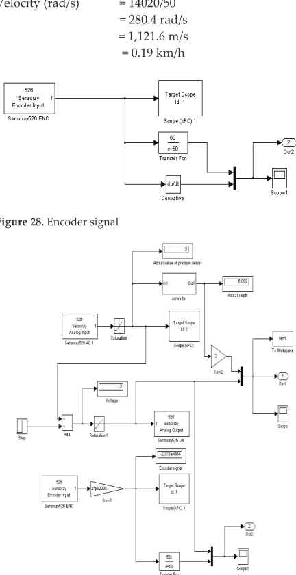
4.5 Encoder signal
This experiment will use an encoder signal to derive the speed of the thrusters, as shown in Figure 28. For distance, the degree will have to be converted to radian by using 2*pi/2000.
To obtain the speed of the thrusters:
Velocity (rad/s) = 14020/50 = 280.4 rad/s = 1,121.6 m/s = 0.19 km/h
Figure 28. Encoder signal
As shown in Figure 29, the complete open loop system for
thrusters is implemented in ROV. The depth is set to
6.082 m with 3V for the pressure sensor. The voltage
applied to the thrusters is 13V. Figure 30 shows the graph for the open loop system.
(a)
(b)
Figure 30. (a) (b) Open loop results
5. System Identification
By using commands in the MATLAB command window,
the input and output will be set. Then the system
identification toolbox interface is opened, as shown in
Figure 31.
>> t=tg.TimeLog; >> R=tg.OutputLog(:,1); >> Y=tg.OutputLog(:,2); >> S=tg.OutputLog(:,3); >> X=tg.OutputLog(:,4); >> ident
where R,Y,S and X are the inputs and outputs of the
system, for example, R for input and Y for output, as
shown in Figure 32. Command “ident” was used to open
the system identification toolbox.
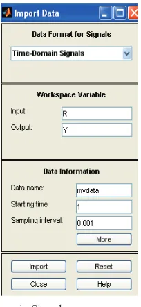
In the “Import data” drop down list, select Time Domain
Data and input, output, starting time and sampling
interval as shown in Figure 31. Then, “Import to SI
toolbox” will be displayed as mydata, as shown in Figure 32. We can set more than one input and output data. But we must remember that the data that we want to analyse
should be highlighted, and the lines of data will be
bigger.
Figure 31. System Identification toolbox
Figure 32. Time Domain Signal
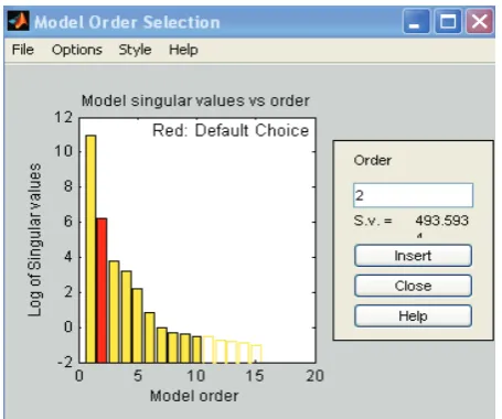
Under the “Estimate” drop‐down list, linear parameter model GUI was selected, as shown in Figure 33. In Linear parameter model GUI, a model other than state‐ space, such as the ARX model, can also be selected. The range of order selected was from 1 to 10, as displayed in Figure 34. Normally the red lines are the default choice. For the thruster used, the second order was selected.
Figure 34. Model order selection
MATLAB Command was used to generate transfer functions model from the state space method for the designed thruster model, at the surface and submerged. This model was based on an open loop model. As the next step, the controller was designed to follow the set point. A Proportional Controller will be used first in this project.
Transfer function:
���� ���������
where X(s) is the input signal with the set point for input depth, while Y(s) is the output signal of the system, which is voltage applied to thrusters corresponding to the input depth [12 ‐ 13].
���� ������������������������������������� (12)
5.1 Comparing Different Models
Based on SI, different models can also be used, instead of only using state space modelling. Here, different modelling was used to come up with thruster models shown in Figure 35 and Figure 36. These represent two different methods to produce the thruster models, where the data can also be converted into transfer function.
Figure 35. ARX model
Figure 36. AMX2221 model
6. Closed Loop System
6.1 Simulation
After the system identification process, the model of the thrusters is developed and a closed loop system is applied. In the first trial, only simulation for the model from SI will be implemented, as shown in Figure 37. Figure 38 shows the input and output system response.
Figure 37. Closed loop system
Figure 38. Input and output of the system response
6.2 Real Time
After the system identification process, the model of the thrusters is developed and a closed loop system is applied. For the first trial, only a real‐time system without a model will be implemented, as shown in Figure 39. The controller uses a conventional proportional controller with the value of gain set to 1 for the first trial in real time. Even using a proportional controller, this gives the best results in a real‐time process.
Figure 39. Closed‐loop system using P controller
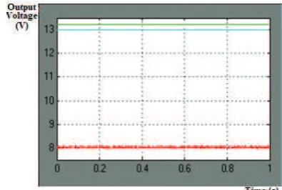
Figure 40 shows the closed loop system with the thrusters model. The transfer function of thrusters is based on Equation (12). Figure 41 and Figure 42 show graphs of the results. The red line is the pressure sensor reading. Here the pressure from the compressor will act as pressure to measure depth. The set point is equal to 13V. The speed of thrusters will be varied by following a very small amount of voltage. For a start, the thrusters will use 13.22V to thrust until the set point of 3V is reached, which is equivalent to 6.082 metres. When the set point is reached the voltage of the thrusters will be constant at 13.1V, which is almost the same as the set point. Meanwhile, Figure 43 shows the initial operation testing in real time of the model thruster. It is shown that at the initial stage no pressure is applied to the pressure sensor. The pressure sensor is maintained at zero depth. Figure 42 on the other hand shows operation testing. In these results the saturation block for motor (thruster) and pressure set the limitation ranges.
Figure 40. Closed loop system with model of thrusters
Figure 41. Initial operation
7. Conclusion
By using system identification, the thruster can be modelled. It is an easier and faster alternative for modelling compared to design by using derivation of mathematical equations. The MPX4250A/MPXA4250A series Manifold Absolute Pressure (MAP) sensor can act as pressure sensor and is suitable to be used for underwater vehicles, especially the ROV used in this project. Different prototypes of ROV will yield different models with the system identification technique because of different parameters like mass, centre of gravity, and gratitude to Universiti Teknikal Malaysia Melaka (UTeM) and Universiti Teknologi Malaysia (UTM), especially to the Faculties of Electrical Engineering, for providing the financial as well as the moral support to complete this project successfully.
9. References
[1] F.A. Azis, M.S.M. Aras, S.S. Abdullah, M.Z.A. Rashid, M.N. Othman. Problem Identification for Underwater Remotely Operated Vehicle (ROV): A Case Study. Procedia Engineering. 2012; 41: pp. 554– 560.
[2] M.S.M. Aras, F.A. Azis, M.N. Othman, S.S. Abdullah. A Low Cost 4 DOF Remotely Operated Underwater Vehicle Integrated with IMU and Pressure Sensor. In: 4th International Conference on Underwater System Technology: Theory and Applications (USYSʹ12). Malaysia. 2012; pp. 18–23.
[3] J.D. Geder, J. Palmisano, R. Ramamurti, W.C. Sandberg, B. Ratna. Fuzzy Logic PID Based Control Design and Performance for a Pectoral Fin Propelled Unmanned Underwater Vehicle. International Conference on Control, Automation and Systems. Seoul, Korea. 2008; pp. 1–7.
[4] Technical Data for Microbox 2000/2000C User’s Manual (xpc target machine), TeraSoft Inc.
[5] C.S. Chin, S.H. Lum. Rapid modeling and control systems prototyping of a marine robotic vehicle with model uncertainties using xPC target system. Ocean Engineering, Elsevier, Amsterdam, The Netherlands, 2011; 38 (17‐18). pp. 2128–2141.
[6] T.H. Koh, M.W.S. Lau, E. Low, G. Seet, S. Swei, P.L. Cheng. A Study of the Control of an Underactuated Underwater Robotic Vehicle. In: Proceedings of the 2002 IEEE/RSJ Intl. Conference on Intelligent Robots and Systems EPFL, Lausanne, Switzerland. 2002; pp. 2049 –2054.
[7] T.I. Fossen. Guidance and control of ocean vehicles, Wiley, New York, 1994.
[8] Freescale Semiconductor Technical Data, Integrated Silicon Pressure Sensor On‐Chip Signal Conditioned, Temperature Compensated and Calibrated MPX4250A /MPXA4250A series Manifold Absolute Pressure (MAP) sensor.
[9] M.S.M. Aras, F. A. Azis, S.M.S. Hamid, F.A. Ali, S.S. Abdullah. Study of the Effect in the Output Membership Function when Tuning a Fuzzy Logic Controller. In: IEEE International Conference on Control System, Computing and Engineering (ICCSCE 2011) Penang, Malaysia, 2011; pp. 1–6. [10] K. Ishaque, S.S. Abdullah, S.M. Ayob, Z. Salam. A
simplified approach to design fuzzy logic controller for an underwater vehicle. Ocean Engineering, Elsevier Amsterdam, The Netherlands. 2010; pp 1 – 14.
[11] K. Ishaque, S.S. Abdullah, S.M. Ayob, Z. Salam. Single Input Fuzzy Logic Controller for Unmanned Underwater Vehicle. In: Journal Intelligence Robot System 2010, 59: pp. 87–100.
[12] Z. Tang, Luojun, Q. He. A Fuzzy‐PID Depth Control Method with Overshoot Suppression for Underwater Vehicle. In: K. Li et al. (Eds.): LSMS/ICSEE 2010, Part II, LNCS 6329. Springer‐Verlag Berlin Heidelberg. 2010; pp. 218–224.
[13] G.V. Nagesh Kumar, K.A. Gopala Rao, P.V.S Sobhan, D. Deepak Chowdary. Robustness of Fuzzy Logic based Controller for Unmanned Autonomous Underwater Vehicle. In: IEEE Region 10 Colloquium and the Third International Conference on Industrial and Information Systems. Kharagpur, India, IEEE, 2008; pp. 1–6.
[14] S.M. Savaresi, F. Previdi, A. Dester, S. Bittanti. Modeling, Identification, and Analysis of Limit‐ Cycling Pitch and Heave Dynamics in an ROV. In: IEEE Journal of Oceanic Engineering. 2004; 29(2): pp. 407–417.
[15] F. Song and S.M. Smith. Combine Sliding Mode Control and Fuzzy Logic Control for Autonomous Underwater Vehicles. In: Advanced Fuzzy Logic Technologies in Industrial Applications 2010; Chapter 13, pp. 191–205.