!" #$ "# #% &$ '#& ($&") * ( + &( & #"*+ * ( ( &(#
,-.. Departement of Statistics
Faculty of Mathematics and Natural Sciences Bogor Agricultural University, Indonesia
E mail: [email protected]
! *" *
A research group on geoinformatics was built in 2010 at Department of Statistics of Bogor Agricultural University, Indonesia, to implement statistical analysis on spatial data. The initial step was to compile some statistical methods related on geographical regression of the simple approach and the complex ones. The methods were implemented to analyse the poverty data in Indonesia. Outcome of selected models was on poverty indicators in a district, such as percentage, expenditure per capita. The outcome was a priory influenced by some regional factors, i.e. local government policy, agro*climate typology, as well as local socio*culture. Therefore, the type of data may produce problems of outliers, outcome dependency, and non*stationarity. Classical approaches assuming there is no effect of the regional differences are not valid any more. For the first phase, the group then implemented methods related on GWR (Geographically Weighted Regression) including simultaneously or conditionally autoregressive models. To obtain firm statistical conclusion, the selected models were contrasted to the ordinary regression. The result indicated that district or regions affected on the poverty level. Hence, spatial factors cannot be neglected in analysing poverty in Indonesia. Additionally, geographical regression performed better than the ordinary models.
Keywords: geographicall regression, regional factors, non*stationarity, spatial data
(*"& / * &(
from place to place. In addition, the usual object of study is spatial unit comprising individuals or household in specific places. These conditions will inevitably introduce the problems of spatial heterogeneity, spatial non*stationarity, and spatial dependency in which the data are obtained. Spatial heterogeneity violates the assumption of variance homogeneity of model residuals (see for example in Getis and Ord, 1992) termed as error propagation by Haining (2004; Section 4.1.3). Spatial non*stationarity causes non* representativeness of global regression models explained nicely by Fotheringham, Brunsdon and Charlton (2002). Spatial dependency violates the assumption of residual independence of regression models. In brief, standard statistical approaches are not appropriate any more and need some adjustment in analyzing spatial data. Otherwise, the models will produce misleading conclusion and recomendation. Anselin and Sergio (2010) provide a comprehensive review of literature on spatial statistics encompasing spatial analysis, pattern analysis, local statistics, and application. Spatial data analysis is commonly implemented in the regional science which includes economic, epidemiology, public health, and environmental sciences. Haining (2004) provide an excelent book related on the teory and practice of spatial data analysis.
Indonesia lies between latitudes 11°S and 6°N with longitudes 95°E and 141°E, a large country with 497 regencies and administrative cities spread out in 33 provinces. The variability of spatial data cannot be avoided due to the natural factors as well as non* natural ones including the local goverments. The local goverments in Indonesia since 2000, according the national regulation, have obtained their autonomy to govern the local programs except for the international policies. Therefore, the local policies will inevitably induce variabilities of some socio*economic variables. In brief, applying adequate methods related to spatial data is getting crucial in the country. Therefore the Department of Statistics of Bogor Agricultural Univesitity has initiated to run research an development in spatial statistics under a group named Geoinformatics. The objectives are to compile, to develop, and to implement spatial statistics in poverty data in Indonesia. Poverty data is an appropriate example for applying spatial statistics as the poverty is affected by the natural and non*natural factors. The term of geoinformatics is interchangably used with spatial stitistics or geo*statistics. However, the GIS (Geographic Information System) part is not elaborated deeply in the paper making a more complit defintion of geoinformatics according to Patil (2005) is not fully followed. The approach is concentrated on statistical modeling and analysis.
analysis) in which ‘location’ factor is included in the analysis (Haining, 2004). The ESDA is then very useful to firstly rcognized the characteristics of data in a specific regions or factors related to the location (space). However, more detail analysis related to statistical relationship, cause*effect models, and prediction are not facilitated in the EDA or ESDA. Davenport and Harris (2008) mention that the more complicated the problems the more statistical intelligent is needed, including statistical analysis and modeling. However, descriptive statistics in EDA/ESDA is still a prerequisite for advances statistics.
"# ) ( "+ "# / *
In this section preliminary results related to standard spatial statistcis are described, i.e. descriptive statistics, geographycally regression and autoregressive models for spatial data. The rest of the approaches are covered partially in the section of model development. The more complex models related to overdispersion, random effect models, and spatial generalized linear models are not elaborated yet in this paper. Hence the paper concentrates on simple approach but very important to consider.
1
' 3 4 % 3 . " 3
In regional based modelling, the ordinary regression (OR) models provides global parameter estimates (ββββs) assuming there is no spatial variation over regions, i.e. spatial stationarity. Unfortuantely, if the assumption is not fulfilled by empirical data, i.e. spatial non*stationarity, the global estimates will not be reliable. Theoretically the paremeter estimates are unbiased and applicable universally to all areas of study. Also, the models do not provide specific parameter estimates depending on the locations. However, geographically Weighted Regression (GWR) is relatively a new alternative approach to construct model on spatial non*stationarity condition (Brunsdon, Fotheringham and Charlton 1996, 1999; Fotheringham, Brunsdon and Charlton 2002). This approach is applied to test the structural stability of the predictors over region because data non* stationarities can compromise global result (Lambert, McNamara and Garrett 2006). By using GWR, it allows to estimate local models and produce local statistics specifically for every region. Fotheringham, Brunsdon and Charlton (2002) provide detail comparison between global and local estimates which is re*presented in Table 1.
* . Differences between local and global statistics
Global Local
Summarize data for whole region Local disaggregation of global statistics Single*valued statistic Multi*values statistic
Non*mappable Mappable
GIS unfriendly GIS friendly
Aspatial or spatially limited Spatial
Emphasize similarities across space Emphasize differences across space Search for regularities or ‘laws’ Search for exceptions or local ‘hot*spots’ (Source : Fotheringham, Brunsdon and Charlton, 2002, pp. 6)
Suppose, response variable of n observations of is formed as a linear function of p predictors. In OR, the model will be generally expressed as
0 1
p
i k k ik i
y =
β
+∑
=β
x +ε
(1)where yi is the outcome of ith observation, xik is i th observation of kth predictors, βk, is k*th regression parameters (k=1, 2,⋯,p) and εi is error term that follows normal distribution with zero mean and known standard deviation and i=1, 2,⋯,n. In matrix notation, if is an n×(p+1) matrix of predictors, is an n×1 column vector of responses, ββββ is an (p+ ×1) 1 column vector of parameter and is column vector of error term, Equation (1) can be written as
OLR model is applied to all regions universally. However, in spatial case, it may be reasonable to assume that the effect of a predictor is conditional upon localized, unobserved factors and social networks (Lambert, McNamara and Garrett 2006). GWR method generates local model for every region, hence spatial effect could be accommodated better than a global model does. GWR is an extension of weighted regression in which the weighting function is based on the relative position among regions. The higher weight is assigned to nearby observation then it will decrease continuously when the distance farther away.
GWR could be applied on linear regression (Brunsdon, Fotheringham and Charlton 1996, 1999, Fotheringham, Brunsdon and Charlton 2002, Propastin, Kappas, and Muratova 2006, Pavlyuk 2009, Shariff, Gairola and Tahib 2010, Rahmawati 2010, Saefuddin, Setiabudi and Achsani 2011), binomial logistic regression (Atkinson, et al 2003, Luo and Wei 2009, Windle et al 2009) and Poisson regression (Nakaya et al 2005, Lambert, McNamara and Garrett 2006). GWR has been applied widely in environment and urban planning (Atkinson et al 2003, Propastin, Kappas, and Muratova 2006, Luo and Wei 2009, Shariff, Gairola, and Tahib 2010), public transportation (Pavlyuk 2009), socio*economic (Brunsdon, Fotheringham and Charlton 1996, Lambert, McNamara and Garrett 2006, Rahmawati 2010), property (Brunsdon, Forteringham, and Chartlon 1999), demographics study (Saefuddin, Setiabudi and Achsani 2011), agriculture and fisheries (Windle et al 2009), epidemiology (Nakaya et al 2005) and many other applications in epidemiology and health. Until now, however, the use of the GWR in Indonesia is very limited. This paper is to review research result related to application of linear GWR on demographic study in Indonesia.
Equation (1) or (2) is considered as global model. Then if linear GWR model is applied, each i*th region of interest will have its own local model expressed as
0( , ) 1 ( , ) p
i i i k k i i ik i
y =
β
u v +∑
=β
u v x +ε
(3)where ( , )u vi i is location of ith observation, or on the other word the centroid of ith region (Fotheringham, Brunsdon and Charlton 2002). Suppose the diagonal elements of an
n n
×
matrix ( , )u vi i consist of the weight at region ( , )u vi i . In matrix notation, for given yi, then1
( T ( , ) ) T ( , )
i i i i i i
y = u v − u v (4)
To define weighting function, there is two common method can be applied, i.e. Gaussian function and bisquare function (Brunsdon, Fotheringham and Charlton 1996; Leung, Mei, and Zhang 2000; Fotheringham, Brunsdon and Charlton 2002). Related to the process of choosing the weighting function, it is very important to predetermine an optimum bandwidth. This could be done by minimizing either cross*validation score or Akaike Information Criteria (Forteringham, Brunsdon and Chartlon 2002).
Regarding to residual sum of squares (RSS), GWR almost performs better than OLR does. However, GWR model needs statistical test to examine whether difference between RSS of GWR and RSS of OLR model, commonly named as GWR improvement, is significant or not. The test is actually to measure goodness*of*fit of GWR model compared to OLR model, that is to test null hypothesis that GWR and OLR model describe data variability equally well against alternative hypothesis that GWR model has better fit than OLR model does. There are several statistical procedures could be employed to perform the examination, i.e. ANOVA or F test (Brunsdon, Forteringham, and Chartlon 1999; Forteringham, Brunsdon and Chartlon 2002), F1 and F2 test (Leung, Mei, and Zhang 2000a). If GWR improvement is statistically significant, test for parameters variability is needed. Leung, Mei and Zhang (2000a) proposed F3 test which takes place in diagnosing whether the set of parameters tend to be constant or to be vary over region. Alternatively, Monte Carlo significance test procedure (Hope 1968) can also be used for such diagnostics.
In Indonesia, the application of the GWR is very limited. However, GWR has been getting implemented and developed, especially by the research group on geoinformatics. This paper presents brief review of GWR application examples in Indonesia which have been presented by the group, i.e. Saefuddin, Setiabudi and Achsani (2011) and Rahmawati (2010), to analyze poverty.
Saefuddin, Setiabudi and Achsani (2011) model poverty as a linear function of Human Development Index (HDI) of 116 districts and administrative cities in Java, Indonesia for the year of 2008 using data from The National Team for Accelerating Poverty Reduction, Office of Vice President of Republic of Indonesia (2010). Due to the existing Java condition, i.e. (1) differences of provincial and district governments, (2) distance of regions to central government, (3) regional autonomy, and (4) differences of agro*ecosystem or climate. Hence, it is reasonable to implement the GWR to analyze relationship between poverty and HDI rather than the OLR.
OLR model of poverty is firstly estimated follows simple linear form of
0 1*
POV =
β
+β
HDI (5)All corresponding pvalues of coefficients in this model indicate that intercept and HDI significantly affect poverty.
* . Parameter estimates of poverty model using OLR
Variable
β
ˆ S( )β
ˆ t Pr(>|t|)Intercept 104.99 8.78 11.95 <.0001
HDI –1.27 0.12 –10.17 <.0001
(Source : Saefuddin, Setiabudi and Achsani, 2011, pp. 281)
Since OLR model seems unsatisfied regarding to RSS and R2, then local models for every point in the region of interest were estimated using GWR. In selecting bandwidth of weighting function, all possible method combinations are utilized and then compared. Finally, the combination of Gaussian function and CV score approach produced an optimum bandwidth. Once, linear GWR was applied using Gaussian weighting function and the optimum bandwidth RSS decreased to 1376.66, R2 increased to 76%, and AICc and AIC decrease to 661.38 and 633.92 respectively.
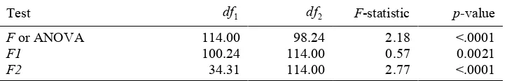
To test GWR improvement, three methods of goodness*of*fits test are performed. Table 3 summaries results of ANOVA or F, F1 and F2 test. According to p values, which were all smaller than 0.05, it could be concluded that that GWR model performed better fits than OLR model did. On the other word, GWR improvement was significant.
* 0. Summary of GWR improvement test for poverty model
Test df1 df2 F*statistic pvalue
F or ANOVA 114.00 98.24 2.18 <.0001
F1 100.24 114.00 0.57 0.0021
F2 34.31 114.00 2.77 <.0001
(Source : Saefuddin, Setiabudi and Achsani, 2011, pp. 282)
Similar to Saefuddin, Setiabudi and Achsani (2011), Rahmawati (2010) previously compared OLR and GWR model of per*capita expenditure per month (EXPE) of 35 villages in regency of Jember, East Java, Indonesia as a function of socio*economic indicators for the year of 2008. Initially, there were 18 predictors selected for the model. However, only three variables were included on the model as a result of variable selection. Those were distance from village to capital of regency (DIST), number of health facility in every 1000 inhabitant (HFAC) and number of beneficiary family of ASKESKIN or health assurance for poor community as percentage of number of total family (ASKES). The general form of global model is
0 1* 2* 3*
* 2. Parameter estimates of expenditure model using OLR
Variable
β
ˆ S( )β
ˆ t Pr(>|t|)Intercept 147313.4 80592.8 1.83 0.077
DIST *2978.2 951.8 *3.13 0.004
HFAC 175907.0 37931.6 4.64 0.000
ASKES *2015.1 739.2 *2.73 0.010
(Source : Rahmawati, 2010, pp. 19)
Fitting an OLR model in the form of equation (6) provides the results in Table 4. According to pvalue on the table, predictors were all significantly affect per*capita expenditure. However, the model above is not quite feasible for use with the R2=64.7% and RSS=16.69 1010.
To improve model accuracy, GWR was applied using both Gaussian and bisquare weighting function. By using Gaussian and bisquare function, RSS decrease to 7 1010 and 8.43 1010 respectively. It seems satisfactory since GWR could reduce residual sum of squares of OLR approximately up to 50%. ANOVA was also performed to examine that this model improvement is significant. Results of ANOVA were listed in Table 5. According to this table, ANOVA result for GWR models using both Gaussian and bisquare weighting function were significant, indicated by p values. This means GWR performed better on describing variability of per*capita expenditure than OLR did.
* 5. Summary of GWR improvement test using ANOVA for per*capita expenditure model
Weighting function df1 df2 F*statistic pvalue
Gaussian 9.70 21.30 3.04 0.020
Bisquare 7.35 23.65 3.15 0.045
In addition, to investigate goodness*of*fits of model, Rahmawati (2010) also calculated Pearson product*moment correlation between observed values of per*capita expenditure to correspond fitted values of OLR and GWR. Table 7 summarized the results.
* 6. Pearson product*moment correlation between observed values of per*capita expenditure to it fitted values
Fitted value r pvalue
OLR model 0.80 0.00
GWR model with Gaussian function 0.92 0.00
GWR model with bisquare function 0.91 0.00
estimates may be ranged from negative to positive. It means a variable could either decrease or increase per*capita expenditure depends on relative position across villages.
According to two illustrations of GWR application above, it is clear in spatial case – but not always – GWR GWR has better performance than OLR. However, if simplicity is a priority, GWR is not to interesting due to model complexity. For governmental policy, the GWR is more preferable to optimally and appropriately allocate limited resources. Hence, regional priorities to be handled can be recommended by GWR analysis. While the OLR one is usually too broad as it does not facilitate the parameter estimates in specific locations.
* 7. Summary statistics of parameter estimates of GWR model of per*capita expenditure
Variable Min Q1 Median Q3 Max Global
Gaussian weighting function
Intercept *171400 14060 42590 207500 562900 147313.4
DIST *8046 *4768 *2745 *1030 3405 *2978.2
HFAC *30150 88950 177400 248900 264700 175907.0
ASKES *3033 *1927 *1735 *901 1097 *2015.1
Bisquare weighting function
Intercept *135000 11250 33100 166600 549800 147313.4
DIST *7322 *4346 *2821 *987 3809 *2978.2
HFAC *32640 81170 218300 246300 262100 175907.0
ASKES *3469 *1920 *1740 *1170 837 *2015.1
(Source : Rahmawati, 2010, pp. 21*22)
0 - 3 1 ) .
The research team also implemented some of the advanced spatial analysis on data assuming dependent on regional factors, i.e. autoregressive models. In this section, a general review was only addressed to Spatial Autoregressive Models (SAR), Spatial Error Models (SEM), and General Spatial Models (SGM). The difference of the three models presented in Table 8. Estimation of parameters in GSM and SAR models were obtained by maximum likelihood approach involving of the areas (Anselin 1988). While the SAR, SEM and SGM are based on the effects of spatial lag (ρ) and spatial error (λ) among areas. Properties and differences of the three spatial methods mentioned above were presented on Table 8.
rejected. In addition, the SAR model It is also performs better than the SEM in the
There are many literatures related to autoregressive models. For examples, Lichstein et al (2002), Tognelli and Kelt (2004), Chun et al (2005), Lee (2005), Kelejian and Prunca (2008) and Mairesse and Mulkay (2008) presented application of SAR models. The example of SEM application could be found at Bhattacharjee and Jensen*Butler (2006) and Benjanuvatra (2009), while GSM at Chun et al (2005).
* . Correlation between HCI of Poverty and Covariates under Study
Covariate Correlation (p < 0.05)
Education Negative (tend to reduce HCI)
Quality of drinking water Negative (tend to reduce HCI) Agricultural work Positive (tend to increase HCI) Non*agricultural work Negative (tend to reduce HCI)
Literacy Non*significant
Type of house Negative (tend to reduce HCI)
8, the null*hypothesises were all rejected at α=5%, indicating that all models were statistically significant and satisfactory. Table 9 showed that the poverty indicated by the HCI was interlinked with covariates. In addition, spatial models performed better the ordinary regression. More detail explanation on the result were available in the master thesis of the team (Meilisa 2010, Yulianto 2011).
0 &( / (' "#) ";
Poverty in Indonesia can be categorized as regionally distributed data. Therefore, spatial statistics is the mode of choice to analyze this kind of data. Geographically Weighted Regression (GWR) performed better than the ordinary regression based on statistical criteria. In addition, the model provides information at each regional model using the local specific models.
The other approaches for regional data are to implement autoregressive models, i.e. Spatial Autoregressive Models (SAR), Spatial Error Models (SEM), and General Spatial Models (SGM) models. These models provide also better conclusion where the error correlation among region are significant. Many other advanced approaches need to be explored in analysing spatial data including Spatial Generalized Linear Mixed Models and Spatial Small Area Estimation. These complex approaches have been being in the progress of research of the group.
2 "#$#"#( #
1. Anselin, L. (1988). Spatial Econometrics: Methods and Models. Dordrecht: Kluwer Academic Publishers.
2. Anselin, L. and Sergio, J.R., Editor. (2010). Perspectives on Spatial Data Analysis. London, UK : Springer.
3. Atkinson, P.M., German, S.E., Sear, D.A. and Clark, M.J. (2003). Exploring the Relations Between Riverbank Erosion and Geomorphological Controls Using Geographically Weighted Logistic Regression. Geographical Analysis, 35(1), 58*82. 4. Benjanuvatra, S. (2009). Comparison of Estimators for Spatial Error Models.
Unpublished paper. York, UK : University of York.
5. Bhattacharjee, A. and Jensen*Butler, C. (2006). Estimation of the Spatial Weights Matrix in the Spatial Error Model, with an Application to Diffusion in Housing Demand. Unpublished paper. St. Andrews, UK : University of St. Andrews.
7. Brunsdon, C., Fotheringham, A.S. and Charlton, M. (1999). Some Notes on Parametric Significance Tests for Geographically Weighted Regression. Journal of Regional Science, 39 (3), 497*524.
8. Chun, D., Jing, H., Wu, X. and Wang, G. (2005). The Study on Spatial Statistics and Its Application in the Spatial Distribution and Evolvement Rule of Radio and TV Industry. Proceedings of the International Symposium on Spatio temporal Modeling, Spatial Reasoning, Analysis, Data Mining and Data Fusion, 27*29 August 2005, Peking University, China.
9. Davenport, T.H. and Harris, J.G. (2008). Competing on Analytics: The New Science of Winning. Massachusetts, US : Harvard Business School Press.
10. Fotheringham, A.S., Brunsdon, C., and Charlton, M. (2002). Geographically Weighted Regression : The Analysis of Spatially Varying Relationships. Chichester: UK.
11. Getis, A. and Ord, J.K. (1992). The Analysis of Spatial Association by Use of Distance Statistics. Geographical Analysis, 24, 189*206.
12. Good, I.J. (1983). The Philosophy of Explanatory Data Analysis. Philosophy of Science, 50, 283*295.
13. Haining, R., (2004). Spatial Data Analysis: Theory and Practice. Cambridge, UK : Cambridge University Press.
14. Kelejian, H.H. and Prucha, R. (2008). Specification and Estimation of Spatial Autoregressive Models with Autoregressive and Heteroskedastic Disturbances. CESifo Working Paper, 2448. www.CESifo*group.org/wpT
15. Lambert, D.M., McNamara, K.T. and Garrett, M.I. (2006). An Application of Spatial Poisson Models to Manufacturing Investment Location Analysis. Journal of Agricultural and Applied Economics, 38(1), 105*121.
16. Lee, L. (2005). The Method of Elimination and Substitution in the GMM estimation of Mixed Regressive, Spatial Autoregressive Models. Unpublished paper. Ohio, US: Ohio State University.
17. Lihstein et al. (2002). Spatial Autocorrelation and Autoregressive Models In Ecology. Ecological Monographs, 72(3), 445–463.
18. Luo, J. and Wei, Y.H.D. (2009). Modeling spatial variations of urban growth patterns in Chinese cities: The case of Nanjing. Landscape and Urban Planning, 91, 51–64. 19. Mairesse, J. and Mulkay, B. (2008). An Exploration of Local R&D Spillovers in
France. NBER Working Paper Series, 14552. http://www.nber.org/papers/w14552 20. Meilisa, M. (2010). Simultaneous Autoregressive Model and Conditional
Autoregressive Model on Poverty Analysis in Eastern Java, Indonesia. Master Thesis. Bogor, Indonesia : Graduated School of Bogor Agricultural University. 21. Nakaya, T., Fotheringham, A.S., Brunsdon, C. and Charlton, M. (2005).
22. Patil, G.P. (2005). Geoinformatics Hotspot System (GHS) for Detection, Prioritization and Early Warning. Proceeding of The National Conference on Digital Governments Research, Georgia, USA, 15*18 May 2005, 116*117.
23. Pavlyuk, D. (2009). Statistical Analysis of the Relationship between Public Transport Accessibility and Flat Prices in Riga. Transport and Telecommunication, 10(2), 26–32.
24. Propastin, P.P., Kappas, M. and Muratova, N.R. (2006). Application of Geographically Weighted Regression Analysis to Assess Human*Induced Land Degradation in a Dry Region of Kazakhstan. Proceedings of XXIII FIG Congress, Munich, Germany, October 8*13, 2006.
25. Rahmawati, R. (2010). Geographically Weighted Regression Using Kernel and Bisquare Weighting Function for Poverty Data (Case Study of 35 Villages in Regency of Jember). Master Thesis. Bogor, Indonesia : Graduated School of Bogor Agricultural University.
26. Saefuddin, A., Setiabudi, N.A., and Achsani, N.A. (2011). On Comparison between Ordinary Linear Regression and Geographically Weighted Regression: With Application to Indonesian Poverty Data. European Journal of Scientific Research, 57(2), 275*285.
27. Saefuddin, A., Sitepu, R.K., Lestariningsih, D. and Setiabudi, N.A. (2011). Exploring Poverty Data Based on PODES and PPLS 2008 Data. Unpublished report. Jakarta : The UKP4 Indonesia.
28. Shariff, N.M., Gairola, S. and Talib, A. (2010). Modelling Urban Land Use Change Using Geographically Weighted Regression and the Implications for Sustainable Environmental Planning. Proceedings of the Fifth Biennial Conference of the IEMSS, Ottawa, Canada, July 5*8, 2010, 2, 1249*1260.
29. The National Team for Accelerating Poverty Reduction. (2010). Welfare Indicators Book I : Poverty. Jakarta: The Office of Vice President of RI.
30. Tognelli, M.F. and Kelt D.A. (2004). Analysis of Determinants of Mammalian Species Richness in South America Using Spatial Autoregressive Models. Ecography, 27, 427*436.
31. Windle, M.J.S., Rose, G.A., Devillers, R. and Fortin, M.J. (2009). Exploring Spatial Non*Stationarity of Fisheries Survey Data Using Geographically Weighted Regression (GWR): An Example from the Northwest Atlantic. Oxford Journals, pp. 145*154.