Computing, Information and Control ICIC International c2013 ISSN 1349-4198
Volume9, Number3, March2013 pp. 1233–1244
ROBUST STATE FEEDBACK CONTROL OF UNCERTAIN POLYNOMIAL DISCRETE-TIME SYSTEMS:
AN INTEGRAL ACTION APPROACH
Shakir Saat1,2, Dan Huang3,4 and Sing Kiong Nguang1 1
Department of Electrical and Computer Engineering The University of Auckland
92019 Auckland, New Zealand
[email protected]; [email protected]
2
The University Technical Malaysia Malacca (on Study Leave) Malacca, Malaysia
3
School of Aeronautics and Astronautics
4
Key Laboratory of System Control and Information Processing, Ministry of Education Shanghai Jiao Tong University
No. 800, Dongchuan Rd., Shanghai 200240, P. R. China [email protected]
Received January 2012; revised May 2012
Abstract. This paper examines the problem of designing a nonlinear state feedback controller for polynomial discrete-time systems with parametric uncertainty. In general, this is a challenging controller design problem due to the fact that the relation between Lyapunov function and the control input is not jointly convex; hence, this problem can-not be solved by a semidefinite programming (SDP). In this paper, a novel approach is proposed, where an integral action is incorporated into the controller design to convexify the controller design problem of polynomial discrete-time systems. Based on the sum of squares (SOS) approach, sufficient conditions for the existence of a nonlinear state feed-back controller for polynomial discrete-time systems are given in terms of solvability of polynomial matrix inequalities, which can be solved by the recently developed SOS solver. Numerical examples are provided to demonstrate the validity of this integral action ap-proach.
Keywords: Polynomial discrete-time systems, SOS decomposition, State feedback con-trol, Integral action method
1. Introduction. Most of the systems in this world such as mechanical systems, electri-cal systems, control systems, and biologielectri-cal systems are nonlinear in nature. This explains why nonlinear systems are very important and have attracted many researchers to involve themselves in this field, especially on stability analysis and controller synthesis of nonlin-ear systems [1, 2, 3, 4, 5, 6]. However, unlike its linnonlin-ear systems counterpart, there is a lack of general analysis and synthesis tools available for nonlinear systems.
In the past decade, there have been several developments on the positive polynomial theory, especially on the sum of squares (SOS) theory; see [7, 8, 9, 10]. The existence of this method gives a new dimension for analyzing and synthesizing the nonlinear systems. In [10], the Gram Matrix method is used to transform the Hamiltion-Jacobi equations (HJE), which are NP-hard to solve, into polynomial matrix inequalities (PMIs) [11]. These PMIs can then be solved in polynomial time with the semidefinite programming (SDP) [12, 13]. The SOS optimization approach is actually a complementary to the LMI approach, but in the polynomial form; see the survey paper [14]. In this survey paper,
the author discusses the relationship between the SOS decomposition and Hilbert’s 17th problem and the positivity of a polynomial under polynomial constraints. Currently, there exist several freely available toolboxes to formulate SOS problems in Matlab, for example SOSTOOLS [15], YALMIP [16], CVX [17] and GLoptiPoly [18].
Recently, several control design approaches based on the SOS decomposition have been proposed for polynomial systems [19, 20, 21, 22, 23, 24]. However, in order to overcome the non-convex terms that exist between the Lyapunov function and the control input, the Lyapunov function must be of a certain structure. More precisely, the Lyapunov function can only depend on the system’s states whose corresponding rows in the control matrix are zeros. This means the states dynamics are not directly affected by the control input, which leads to conservative results. To overcome this conservatism, in [20, 21], a pre-defined upper bound is used to bound the non-convex term that exists between the Lyapunov function and the control input. However, this pre-defined bound is hard to determine beforehand, and the closed-loop stability can only be guaranteed within a bound region. Other attempts in the area of polynomial systems stabilization can be found in [25, 26]; however, their results are also held locally. The SOS method has also been applied in the T-S fuzzy model frameworks [27].
When it comes to the controller synthesis for polynomial discrete-time systems, there are only few results available which utilize SOS decomposition method. This is due to the fact that the relation between Lyapunov functions and controller matrices is always not jointly convex. Hence, it is hard to solve for a Lyapunov function and controller matrices simultaneously. This problem does not exist if the Lyapunov function is in the quadratic form. Recently, some attempts have been made to overcome this problem. In [28, 29], following the same approach as [20, 21], the non-convex term is assumed to be bounded by a pre-defined upper bound. For the same reason, they share the same weaknesses as [20, 21].
Motivated by the aforementioned problem, we propose a new technique to deal with the nonconvex terms that exist between the Lyapunov function and the control input. In our work, in order to transform the state feedback controller design problem into a tractable SDP, the integral action is incorporated into the controller design. In doing so, we manage to convexify the problem and it consequently can be solved by the SDP. In comparison with the existing method of state feedback control designs for polynomial discrete-time systems [29], there are three features of our proposed approach deserving attention. First, our method yields a robust stabilizing state feedback controller for polynomial discrete-time systems with polytopic uncertainties. Second, with the existence of integral action in the controller designs, the non-convex terms can be efficiently eliminated, hence relax the conservatism issue that encountered in [29]. Finally, the Lyapunov function does not need to be of a special form to render a convex solution. For that reason, the proposed method provides a more general and less conservative result than the existing one. Also, to the best of the authors’ knowledge, the problem of the robust state feedback synthesis for polynomial discrete-time systems that utilize the SOS programming has not been fully studied. The main contributions of this paper can be summarized as follows:
• An integral action is introduced into the controller designs to convexify the nonlinear terms that exists in the problem formulation of polynomial discrete-time synthesis.
• The nonconvex terms are not assumed to be bounded as in [29].
• The Lyapunov function does not need to depend on states whose corresponding rows in control matrix are zeros.
Then, the validity of our proposed approach is illustrated using examples in Section 4. Conclusions are given in Section 5.
2. Preliminaries and Notations. In this section, we introduce the notation that will be used in the rest of the paper. Furthermore, we provide a brief review of the SOS decomposition. For a more elaborate description of the SOS decomposition, refer to [10].
2.1. Notations. Let R be the set of real numbers and Rn be the n-dimensional real space. Furthermore, let In represent the identity matrix of size n×n. Q > 0 (Q ≥ 0) is used to express the positive (semi)definiteness of (the square) matrix Q. Also, for simplicity a P(x+) is employed to represent P(x(k+ 1)).
A (∗) is used to represent transposed symmetric matrix elements.
2.2. SOS decomposition.
Definition 2.1. A multivariate polynomial f(x), for x∈Rn is a sum of squares if there
exist polynomials fi(x), i= 1, . . . , m such that
f(x) = m
∑
i=1
fi2(x). (1)
From Definition 2.1, it is clear that the set of SOS polynomials in n variables is a convex cone, and it is also true (but not obvious) that this convex cone is proper [30]. If a decomposition of f(x) in the above form can be obtained, it is clear that f(x) ≥ 0,
∀x∈Rn. The converse, however, is generally not true.
The problem of finding the right-hand side of (1) can be formulated in terms of the existence of a positive semidefinite matrix Q such that the following proposition holds:
Proposition 2.1. [10] Let f(x) be a polynomial in x ∈ Rn of degree 2d. Let Z(x) be a
column vector whose entries are all monomials in x with degree ≤d. Then, f(x) is said to be SOS if and only if there exists a positive semidefinite matrix Q such that
f(x) =Z(x)TQZ(x) (2) In general, determining the non-negativity of f(x) for deg(f) ≥ 4 is classified as an NP-hard problem [31, 32]. However, using Proposition 2.1 to formulate nonnegativity conditions on polynomials provides a relaxation that is computational tractable. A more general formulation of this transformation for symmetric polynomial matrices is given in the following proposition:
Proposition 2.2. [19] Let F(x) be an N ×N symmetric polynomial matrix of degree 2d
in x∈Rn. Furthermore, let Z(x) be a column vector whose entries are all monomials in
x with a degree no greater than d, and consider the following conditions (1) F(x)≥0 for all x∈Rn;
(2) vTF(x)v is a SOS, where v ∈RN;
(3) There exists a positive semidefinite matrix Q such that vTF(x)v = (v⊗Z(x))T
Q(v⊗
Z(x)), with ⊗ denoting the Kronecker product.
It is clear that F(x)being a SOS implies that F(x)≥0, but the converse is generally not true. Furthermore, statement (2) and statement (3) are equivalent.
3.1. Nonlinear state feedback control design. Consider the following dynamic model of a polynomial discrete-time system:
x(k+ 1) =A(x(k))x(k) +B(x(k))u(k)
y(k) =C(x(k))x(k)
}
(3)
wherex(k)∈Rnis a state vector. A(x(k)),B(x(k)) andC(x(k)) are polynomial matrices of appropriate dimensions.
Select a Lyapunov function as
V(x(k)) =xT(k)P−1(x(k))x(k) (4)
where P(x(k)) is defined to be a symmetrical N ×N polynomial matrice whose (i, j)-th entry is given by
pij(x(k)) =p0ij +pijgm(k)(1:l) (5) where i= 1,2, . . . , n, j = 1,2, . . . , nand g = 1,2, . . . , dwhere nis a number of states and
d is total monomials numbers. It is important to note here that m(k) is all monomials vectors in (x(k)) from degree of 1 to degree of l, where l is a scalar even value. For example, if l= 2, and x(k) = [x1(k), x2(k)]T, then p
11 =p11+p112x1+p113x2 +p114x21+ p115x1x2 +p116x2
2. This is a more general structure as compared with [29] because of a
higher value of l, a more relaxation in SOS problem can be achieved. Next, we introduce a state feedback controller as
u=K(x(k))x(k) (6)
For this purpose, we use the standard assumption for the state feedback control where all states vector x(k) are available for feedback. Then, with (3) and the state feedback controller as described in (6), the following theorem is established.
Theorem 3.1. The system (3) is asymptotically stable if
1. There exist positive definite symmetric polynomial matrix, P(x(k)) and polynomial matrix, K(x(k)) such that
−(A(x(k))+B(x(k)K(x(k))))TP−1(x
+)(A(x(k))+B(x(k))K(x(k)))+P−1(x(k))>0 (7)
or
2. There exist positive definite symmetric polynomial matrix, P(x(k)), polynomial ma-trices, K(x(k)) and G(x(k)) such that
[
G(x(k)) +GT(x(k))−P(x(k)) ∗
A(x(k))G(x(k)) +B(x(k))K(x(k))G(x(k)) P(x+)
]
>0. (8)
Proof: We begin proving (7) is asymptotically stable by taking the difference between
V(x(k+ 1)) and V(x(k)) along (3). Thus producing
∆V(x(k)) =xT(x(k+ 1))P−1(x
+)x(x(k+ 1))−xT(k)P−1(x(k))x(k)
=(
A(x(k))x(k) +B(x(k))K(x(k))x(k))T
P−1(x
+)(A(x(k))x(k)
+B(x(k))K(x(k))x(k))−xT(k)P−1(x(k))x(k)
=xT(k)[(AT(x(k)) +KT(x(k))BT(x(k)))P−1(x
+)(A(x(k)) +B(x(k))K(x(k)))
−P−1(x(k))]x(k) (9)
From [2] if (4) is >0 and
(
AT(x(k)) +KT(x(k))BT(x(k)))
P−1(x
holds, then the system (3) with (6) is globally asymptotically stable. The equivalence between Statement 1 and 2 come from the Finsler’s Lemma; hence the proof is omitted here.
Remark 3.1. The introduction of a new matrix variable, G(x(k)), provides a great ad-vantage in the analysis of nonlinear polynomial systems. This approach was introduced in [33] for linear cases, and has been adopted by [29] for nonlinear cases. Generally, for nonlinear cases the main advantage of introducing this new matrix variable is that the selection of a polynomial feedback control law can be chosen to be a polynomial of ar-bitrary degree, which improves the solvability of the nonlinear matrix inequalities by the SOS solver. Note that this extra matrix is not constrained to be a symmetric polynomial matrix.
It is worth mentioning that the conditions given in Theorem 3.1 are in terms of state dependent BMIs. Thus, solving this inequality is computationally hard because it needs to solve an infinite set of state-dependent LMIs. To relax these conditions, we utilize the SOS decomposition approach as described in [10] and have the following proposition:
Proposition 3.1. The system (3) is asymptotically stable if there exist a symmetrical polynomial matrix,P(x(k)), polynomial matricesK(x(k))andG(x(k)), a constantǫ1 >0
and a sum of squares polynomial ǫ2(x(k)) such that the following conditions hold for all x(k)6= 0
vT[P(x(k))−ǫ1I]v is a SOS (10)
vT1 [M −ǫ2(x(k))I]v1T is a SOS (11)
where
M =
[
G(x(k)) +GT(x(k)−P(x(k)) ∗
A(x(k))G(x(k)) +B(x(k))K(x(k))G(x(k)) P(x+)
]
(12)
Meanwhile, v and v1 are vectors with appropriate dimensions.
Proof: The proof for this proposition is similar to Theorem 3.1. ∆∆∆ Unfortunately, Proposition 3.1 cannot be solved easily by SDP because the term in
P(x+) is not jointly convex. This situation is explained in the following remark.
Remark 3.2. Let us expand the term, P(x+),
P(x+) =P(x(k+ 1))
=P (A(x(k))x(k) +B(x(k))u(k))
=P (A(x(k))x(k) +B(x(k))K(x(k))x(k)) (13)
From (13), the relation between polynomial matrix, P, and controller matrix, K(x(k)), is not jointly convex; hence it cannot be solved by SDP. This is the main difficulty when designing a controller for polynomial discrete-time systems. Motivated by this fact, we propose a novel approach in which the above-mentioned problem can be removed by having an integral action in the controller designs.
3.2. An integral action approach. In this subsection, we describe in detail our proach for handling the above-mentioned problem. To help readers understand this ap-proach, we re-write (3)
x(k+ 1) =A(x(k))x(k) +B(x(k))u(k)
y(k) =C(x(k))x(k)
}
Furthermore, to stabilize (14), a state feedback controller with an integral action is proposed as follows:
z(k+ 1) =z(k) +f(k)
u(k) =z(k)
}
(15)
where f(k) is a new control input to the system. Using (15), (14) can be transformed into augmented systems as follows:
ˆ
x(k+ 1) =
[
x(k+ 1)
z(k+ 1)
]
=
[
A(x(k))x(k) +B(x(k))z(k)
z(k) +f(k)
]
(16)
or
ˆ
x(k+ 1) =
[
A(x(k)) B(x(k))
0 1
]
ˆ
x(k) +
[
0 1
]
f(k) (17)
Selecting f(k) = ˆf(ˆx(k))ˆx(k), (17) can be rewritten in the following compact form:
ˆ
x(k+ 1) = ˆA(ˆx(k))ˆx(k) + ˆB(ˆx(k)) ˆf(ˆx(k))ˆx(k) (18)
where
ˆ
A(ˆx(k)) =
[
A(x(k)) B(x(k))
0 1
]
and Bˆ(ˆx(k)) =
[
0 1
]
Then, a Lyapunov function is selected to be ˆ
V(ˆx(k)) = ˆxT(k) ˆP−1(x(k))ˆx(k) (19) Remark 3.3. The interesting part of the Lyapunov function in (19)is that the polynomial matrix, Pˆ(x(k))is only dependent upon the original system states,x(k). By employing this kind of representation, we can avoid the existence of nonconvex terms in our formulation. The validity of this statement is given next.
From (19), the difference between ˆV(ˆx(k+ 1)) and ˆV(ˆx(k) can be written as
∆ ˆV(ˆx(k)) = ˆx(k+ 1)TPˆ−1(x
+)ˆx(k+ 1)−xˆT(k) ˆP−1(x)ˆx(k)
=(ˆ
A(ˆx(k))ˆx(k) + ˆB(ˆx(k)) ˆf(ˆx(k))ˆx(k))T ˆ
P−1(x
+)( ˆA(ˆx(k))ˆx(k)
+ ˆB(ˆx(k)) ˆf(ˆx(k))ˆx(k))
−xˆT(k) ˆP−1(x)ˆx(k)
= ˆxT(k)[(ˆ
AT(ˆx(k)) + ˆfT(ˆx(k)) ˆBT(ˆx(k)))ˆ
P−1(x
+)
(ˆ
A(ˆx(k)) + ˆB(ˆx(k)) ˆf(ˆx(k))
−Pˆ−1(x(k))]xˆ(k) (20)
Remark 3.4. It is obvious from (20) that system (18) can be stabilized by (15) if we can guarantee (19) is >0 and
[(ˆ
AT(ˆx(k)) + ˆfT(ˆx(k)) ˆBT(ˆx(k)))ˆ
P−1(x
+)
(ˆ
A(ˆx(k)) + ˆB(ˆx(k)) ˆf(ˆx(k))
−Pˆ−1(x(k))] <0
(21)
From (21), we use the procedure as highlighted in Theorem 3.1 and adopt the [33] approach, which yields
[ ˆ
G(ˆx(k)) + ˆGT(ˆx(k))−Pˆ(x(k)) ∗ ˆ
A(ˆx(k)) ˆG(ˆx(k)) + ˆB(ˆx(k)) ˆf(k) ˆG(ˆx(k)) Pˆ(x+)
]
>0 (22)
Now, defining ˆL(ˆx(k)) = ˆf(ˆx(k))G(ˆx(k)), (22) becomes
[ ˆ
G(ˆx(k)) + ˆGT(ˆx(k))−Pˆ(x(k)) ∗ ˆ
A(ˆx(k)) ˆG(ˆx(k)) + ˆB(ˆx(k)) ˆL(ˆx(k)) Pˆ(x+)
]
Remark 3.5. Note that Pˆ(x+) does not contain the controller matrix, because Pˆ(x(k))
is a function of x(k) only. Basically, Pˆ(x+) = ˜pij(A(x(k))x(k) +B(x(k))z(k)), where ˜
pij =p0ij+pijg as described in (5). Note thati= 1,2, . . . , nandj = 1,2, . . . , n. Therefore, (23) can be solved efficiently by SDP because the terms there are convex.
Sufficient conditions for the existence of our proposed controller are given in the fol-lowing proposition:
Proposition 3.2. The system (14)is stabilizable via the state feedback control in the form of (15) if there exists a symmetrical polynomial matrix, Pˆ(x(k)), polynomial matrices
ˆ
L(ˆx(k)) and Gˆ(ˆx(k)), a constant ǫ1 >0, and a sum of squares polynomial ǫ2(ˆx(k)) such that the following conditions satisfy for all x(k)6= 0
v3T[ ˆP(x(k))−ǫ1I]v3 is a SOS (24) vT4 [M1−ǫ2(ˆx(k))I]v4 is a SOS (25)
where
M1 =
[ ˆ
G(ˆx(k)) + ˆGT(ˆx(k))−Pˆ(x(k)) ∗ ˆ
A(ˆx(k)) ˆG(ˆx(k)) + ˆB(ˆx(k)) ˆL(ˆx(k)) Pˆ(x+)
]
(26)
Meanwhile, v3 and v4 are vectors with appropriate dimensions.
3.3. Robust state feedback control design. The results presented in the previous section assume that the system’s parameters are known exactly. In this section, we investigate how the above method can be extended to systems in which the parameters are not exactly known.
Consider the following system
x(k+ 1) =A(x(k), θ)x(k) +B(x(k), θ)u(k)
y=Cy(x(k), θ)x(k)
(27)
where the matrices ·(x(k), θ) are defined as follows:
A(x(k), θ) = q
∑
i=1
Ai(x(k))θi,
B(x(k), θ) = q
∑
i=1
Bi(x(k))θi,
Cy(x(k), θ) = q
∑
i=1
Cyi(x(k))θi
(28)
θ =[
θ1, . . . , θq
]T
∈Rq is the vector of constant uncertainty and satisfies
θ ∈Θ,
{
θ∈Rq :θi ≥0, i= 1, . . . , q, q
∑
i=1
θi = 1
}
. (29)
We further define the following parameter-dependent Lyapunov function
˜
V(x(k)) = ˆxT(k)
( q ∑
i=1
ˆ
Pi(x(k))θi
)−1
ˆ
x(k), (30)
where ˆP(x(k)) is defined as (19).
Proposition 3.3. Given a constant ǫ1 > 0 and SOS polynomial functions ǫ2(x) > 0
for x 6= 0, the system (27) with the state feedback controller (15) is stable for x 6= 0
and i = 1, . . . , q if there exist common polynomial matrices Gˆ(ˆx(k)) and Lˆ(ˆx(k)) and a symmetrical polynomial matrix, Pˆi(x(k)) such that the following conditions hold
vT
5[ ˆPi(x)−ǫ1I]v5 is a SOS (31)
v6T [M2−ǫ2(x(k))I]v6 is a SOS (32)
where
M2 =
[ ˆ
G(ˆx(k)) + ˆGT(ˆx(k))−Pˆi(x(k)) ∗ ˆ
Ai(ˆx(k)) ˆG(ˆx(k)) + ˆBi(ˆx(k)) ˆL(ˆx(k)) Pˆi(x+)
]
(33)
Proof: This proposition follows directly as a convex combination of several systems of
the form (3) for a common (15). ∆∆∆
4. Numerical Examples. In this section, we provide several design examples to demon-strate the validity of our proposed approach.
4.1. Without uncertainty.
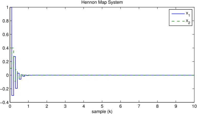
Example 4.1. Hennon Map Systems Consider the following Hennon Map system,
x(k+ 1) =
[
−ax21(k) +x2(k) + 1 bx1(k) + 0
]
+
[
1
c
]
u, (34)
where a = 1.4 and b = 0.3. With this specification, the Hennon map behaves chaotically. In this work, c value is chosen as 0.1. With the introduction of an integral action, it can be written as
ˆ
x(k+ 1) =
−ax1 1 1 b 0 c
0 0 1
x1(k) x2(k) z(k)
+
0 0 1
f(k) +
1 0 0
. (35)
Next, we chooseǫ1 = 0.01andǫ2(x) = 0.0001 (x2
1(k) +x22(k) +z2(k)). Using the procedure
described in Proposition 3.2, and with the degree of Pˆ(x(k)) and Gˆ(ˆx(k)) being in degree of 4 and Lˆ(ˆx(k)) being chosen to be in the degree of 8, a feasible solution is achieved. The simulation result has been plotted in Figure 1 for initial value [x1, x2] = [1,1]. From Figure 1, the controller stabilizes the system states to the desired operating region.
Remark 4.1. It is important to highlight here that using the approach proposed by [29], no solution could be obtained for this example. This confirms that our approach is less conservative than [29].
4.2. With parametric uncertainty. This section illustrates the results of a state feed-back control for polynomial discrete-time systems with polytopic uncertainties.
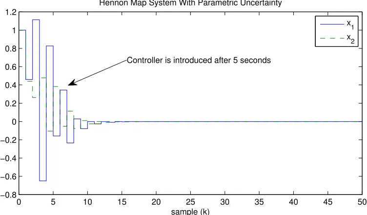
Example 4.2. Hennon Map System The dynamics of the Hennon Map system is described as follows:
x(k+ 1) =
[
−ax21(k) +x2(k) + 1 bx1(k) + 0
]
+
[
1
c
]
u(k), (36)
0 1 2 3 4 5 6 7 8 9 10 −0.4 −0.2 0 0.2 0.4 0.6 0.8 1
Hennon Map System
sample (k)
x
1
x
[image:9.595.112.488.84.303.2]2
Figure 1. State feedback control for Hennon Map witha = 1.4 and b= 0.3
change from their nominal values in its parameter. Then, (36) can be written in the form of upper, xU(k+ 1) and lower bounds, xL(k+ 1) as below:
xU(k+ 1) =
[
−a+ (0.1a) 1
b+ (0.1b) 0
] [
x1(k)
x2(k)
]
+
[
1
c+ (0.1c)
]
u(k) +
[
1 0
]
xL(k+ 1) =
[
−a−(0.1a) 1
b−(0.1b) 0
] [
x1(k)
x2(k)
]
+
[
1
c−(0.1c)
]
u(k) +
[
1 0
]
(37)
Then, applying a proposed approach as described in a preceding section,(37)can be written as an augmented system as below:
ˆ
xU(k+ 1) =
−a+ (0.1a) 1 1
b+ (0.1b) 0 c+ (0.1c)
0 0 1
x1(k)
x2(k) z(k)
+ 0 0 1
f(k) + 1 0 0 ˆ
xL(k+ 1) =
−a−(0.1a) 1 1
b−(0.1b) 0 c−(0.1c)
0 0 1
x1(k)
x2(k)
z(k)
+ 0 0 1
f(k) + 1 0 0 (38)
Next, we select ǫ1 = 0.01 and ǫ2(x) = 0.0001 (x12(k) +x22(k) +z2(k)). Furthermore,
im-plementing the procedure outlined in Proposition 3.3, we initially choose the degree of the
ˆ
P1(x(k)) and Pˆ2(x(k)) to be 2. The common polynomial matrices Gˆ(ˆx(k)) and Lˆ(ˆx(k))
are also selected to be in the degree of 2, but no feasible solution can be achieved. Then, the degree of Pˆ1(x(k)),Pˆ2(x(k)), Gˆ(ˆx(k)) are increased to 4. Meanwhile, the degree of
ˆ
L(ˆx(k)) is increased to 8, and with this arrangement a feasible solution is obtained. The simulation results for this example are given in Figure 2 between two vertices of (38)with the initial condition of [1 1]. It is obvious from Figure 2, our proposed controller sta-bilizes the system well. It is also important to note that the controller is only introduced after 5s.
0 5 10 15 20 25 30 35 40 45 50 −0.8
−0.6 −0.4 −0.2 0 0.2 0.4 0.6 0.8 1 1.2
Hennon Map System With Parametric Uncertainty
sample (k)
x
1
x
2
[image:10.595.110.486.86.306.2]Controller is introduced after 5 seconds
Figure 2. State feedback control for Example 4.2
5. Conclusions. This paper has examined the problem of designing a state feedback con-troller for polynomial discrete-time systems with polytopic uncertainties using a parame-ter-dependent Lyapunov functions. More precisely, a state feedback controller with an integral action is proposed to stabilize the polynomial discrete-time systems. By introduc-ing an integral action into the controller designs, an original system can be transformed into an augmented system. Through this, a nonconvex controller design problem can be converted into a convex controller design problem, hence can be solved by SDP effi-ciently. In addition, the nonconvex terms, P(x(k+ 1)) are not assumed to be bounded as in [29]. Hence, this methodology provides a more general and less conservative result than available approaches in the similar underlying problem. The existence of the state feedback controller with an integral action is given in terms of solvability conditions of the polynomial matrix inequalities (PMIs), which formulated as SOS constraints. Numerical examples have been provided to demonstrate the validity of this integral action approach.
Acknowledgement. This work is partially supported by the University of Malaysia Malacca, Malaysia (UTeM), Malaysia Government Sponsorship (SLAB), The University of Auckland, The National Natural Science Foundation of China (No. 61004026), and Ph.D. Programs Foundation of Ministry of Education of China (No. Z1025409). The authors also gratefully acknowledge the helpful comments and suggestions of the reviewers, which have improved the presentation.
REFERENCES
[1] P. Kokotovic and M. Arcak, Constructive nonlinear control: A historical perspective,Automatica, vol.37, no.5, pp.637-662, 2001.
[2] H. K. Khalil, Nonlinear Systems, Prentice-Hall, 1996.
[3] A. Isodori,Nonlinear Control Systems, Springer-Verlag, 1995.
[4] W. M. Lu and J. Doyle, H∞ control of nonlinear systems: A convex characterization, American
Control Conference, vol.2, pp.2098-2102, 1994.
[5] M. Krstic, I. Kanellakopoulos and P. V. Kokopotic, Nonlinear An Adaptive Control Design, John Wiley and Sons, New York, NY, 1995.
[7] D. Henrion and J. B. Lasserre, Positive polynomials in control,LNCS, vol.312, 2005.
[8] A. Papachristodoulou and S. Prajna, On the construction of Lyapunov functions using the sum of squares decomposition,Conference on Decision and Control, vol.3, pp.3482-3487, 2002.
[9] S. Prajna, P. Parrilo and A. Rantzer, Nonlinear control synthesis by convex optimization, IEEE Transactions on Automatic Control, vol.49, no.2, pp.310-314, 2004.
[10] P. A. Parrilo,Structured Semidefinite Programs and Semialgebraic Geometry Methods in Robustness and Optimization, Ph.D. Thesis, California Institute of Technology, 2000.
[11] V. Powers and T. W¨ormann, An algorithm for sums of squares of real polynomials,Journal of Pure and Applied Algebra, vol.127, no.1, pp.99-104, 1998.
[12] L. Vandenberghe and S. P. Boyd, Semidefinite programming, SIAM Review, vol.38, no.1, pp.49-95, 1996.
[13] S. P. Boyd, L. E. Ghaoui, E. Feron and V. Balakrishnan,Linear Matrix Inequalities in System and Control Theory, SIAM, Philadelphia, 1994.
[14] G. Chesi, LMI techniques for optimization over polynomials in control: A survey, IEEE Transac-tions on Automatic Control, vol.55, no.11, pp.2500-2510, 2010.
[15] S. Prajna, A. Papachristodoulou and P. A. Parrilo, Introducing SOSTOOLS: A general purpose sum of squares programming solver, Conference on Decision and Control, vol.1, pp.741-746, 2002. [16] J. Lofberg, YALMIP: A toolbox for modeling and optimization in Matlab, IEEE International
Symposium on Computer Aided Control Systems Design, pp.284-289, 2004.
[17] M. Grant and S. Boyd, Graph implementations for nonsmooth convex programs, inRecent Advances in Learning and Control, Lecture Notes in Control and Information Sciences, V. Blondel, S. Boyd and H. Kimura (eds.), Springer-Verlag, 2008.
[18] D. Henrion, J. B. Lasserre and J. L¨ofberg, GloptiPoly 3: Moments, optimization and semidefinite programming, Optimization Methods and Software, vol.24, no.4, pp.761-779, 2009.
[19] S. Prajna, A. Papachristodoulou and F. Wu, Nonlinear control synthesis by sum of squares op-timization: A Lyapunov-based approach, The 5th Asian Control Conference, vol.1, pp.157-165, 2004.
[20] H. J. Ma and G. H. Yang, Fault-tolerant control synthesis for a class of nonlinear systems: Sum of squares optimization approach, International Journal of Robust and Nonlinear Control, vol.19, no.5, pp.591-610, 2009.
[21] D. Zhao and J. Wang, An improved H∞ synthesis for parameter-dependent polynomial nonlinear
systems using sos programming,American Control Conference, pp.796-801, 2009.
[22] S. Saat, M. Krug and S. K. Nguang, A nonlinear static output controller design for polynomial systems: An iterative sums of squares approach,The 4th International Conference on Control and Mechatronics, pp.1-6, 2011.
[23] S. Saat, M. Krug and S. K. Nguang, Nonlinear H∞ static output feedback controller design for
polynomial systems: An iterative sums of squares approach,The 6th IEEE Conference on Industrial Electronics and Applications, pp.985-990, 2011.
[24] S. K. Nguang, S. Saat and M. Krug, Static output feedback controller design for uncertain polyno-mial systems: An iterative sums of squares approach,IET Control Theory and Applications, vol.5, no.9, pp.1079-1084, 2011.
[25] Q. Zheng and F. Wu, Regional stabilisation of polynomial nonlinear systems using rational Lya-punov functions, International Journal of Control, vol.82, no.9, pp.1605-1615, 2009.
[26] T. Jennawasin, T. Narikiyo and M. Kawanishi, An improved SOS-based stabilization condition for uncertain polynomial systems,SICE Annual Conference, pp.3030-3034, 2010.
[27] D. Zhang, Q. Zhang and Y. Zhang, Stabilization of T-S fuzzy systems: An SOS approach, In-ternational Journal of Innovative Computing, Information and Control, vol.4, no.9, pp.2273-2283, 2008.
[28] J. Xu, L. Xie and Y. Wang, Synthesis of discrete-time nonlinear systems: A sos approach,American Control Conference, pp.4829-4834, 2007.
[29] H. J. Ma and G. H. Yang, Fault tolerantH∞control for a class of nonlinear discrete-time systems:
Using sum of squares optimization,American Control Conference, pp.1588-1593, 2008.
[30] H. Hindi, A tutorial on convex optimization, American Control Conference, vol.4, pp.3252-3265, 2004.
[31] A. Papachristodoulou and S. Prajna, A tutorial on sum of squares techniques for systems analysis, Proc. of the 2005 American Control Conference, vol.4, pp.2686-2700, 2005.