FUNDAMENTAL DESIGN OF MODEL PREDICTIVE
CONTROLLER, PERFORMANCE STUDIES AND
ANALYSIS
Wan Hazwani Binti Wan Hassan
B010810308
Bachelor of Electrical Engineering
(Control, Instrumentation and Automation)
Supervisor: Datuk Professor Dr. Mohd Ruddin
Bin Ab. Ghani
PERFORMANCE STUDIES AND ANALYSIS
WAN HAZWANI BINTI WAN HASSAN
A report submitted in partial fulfilment of the requirement for the Degree of
Electrical Engineering (Control, Instrumentation and Automation)
Faculty of Electrical Engineering
UNIVERSITI TEKNIKAL MALAYSIA MELAKA
“I hereby declare that I have read through this report entitle “ Fundamental Design
of Model Predictive Controller, Performance Comparisons and Analysis” and found that it
has comply the partial fulfilment for awarding the degree of Bachelor of Electrical
Engineering (Control, Instrumentation and Automation)”
Signature
:
Supervisor‟s Name :
Datuk Professor Dr. Mohd Ruddin Bin Ab. Ghani
DECLARATION
“I declare that this report entitle “Fundamental Design of Model Predictive
Controller, Performance Comparisons and Analysis” is the result of my own research
except as cited in the references. The report has not been accepted for any degree and is not
concurrently submitted in candidature of any other degree”
Signature
:
Name
:
Wan Hazwani Binti Wan Hassan
To my beloved father and mother
ACKNOWLEDGEMENT
First and foremost, i would especially like to devote a great appreciation to my
supervisor, Datuk Professor Dr. Mohd Ruddin Bin Ab. Ghani for his help, advice and
motivation. Not forgetting my former supervisor Mdm. Sazuan Nazrah Binti Mohd Azam
for the ideas, guidance, suggestions and knowledge of controller design and performance
studies, and contributions in completion of this final year project.
I also would like to take this opportunity to express my gratitude to my university,
Universiti Teknikal Malaysia Melaka (UTeM) for giving me the opportunity in my studies.
Thank you to panels, Mr. Hyreil Anuar and Mdm. Ezreen Farina for kindly evaluates my
presentation and demonstration. I would also like to thank my academic advisor and all
lecturers in Faculty of Electrical Engineering for the help, guidance and support. Not
forgetting the lab technician for their help.
My deepest thanks go to my father, Wan Hassan and my mother, Maimunah for
their endless prayer, morally support and patience. To my family and friends for their
endless prayers, encouragement and understanding. To Noraini, Jazli, Hisham and Oon,
thank you for the support and opinions. Special thanks to my beloved friend Faizal for the
support, time and knowledge.
ABSTRACT
ABSTRAK
TABLE OF CONTENTS
CHAPTER TITLE
PAGE
ACKNOWLEDGEMENT
i
ABSTRACT
ii
ABSTRAK
iii
TABLE OF CONTENTS
iv
LIST OF TABLES
vi
LIST OF FIGURES
vii
LIST OF APPENDICES
ix
1
INTRODUCTION
1
1.1
PROBLEM STATEMENT
1
1.2
OBJECTIVES
1
1.3
PROJECT SCOPE
1
2
LITERATURE REVIEW AND THEORY
3
2.1
INTRODUCTION
3
2.2
TEMPERATURE CONTROL
3
2.3
MODELING AND SYSTEM IDENTIFICATION
3
2.3.1 Transfer Function
4
2.4
MODEL PREDICTIVE CONTROLLER
7
2.5
ANALYSIS
9
2.5.1 Transient Response
9
2.5.2 Performance Evaluation
10
2.5.3 Robustness Tests and tuning validation
10
3
METHODOLOGY
12
3.1
INTRODUCTION
12
3.2.1 System Identification
15
3.3
PHASE 2 – CONTROLLER DESIGN
19
3.4
PHASE 3 – ANALYSIS
22
3.4.1 Performance Comparisons
22
3.4.1.1 Step Response 23 3.4.1.2 Set Point Changes 243.4.2 Robustness Tests
25
3.4.2.1 Disturbance Rejection 25 3.4.2.2 Random Set Point Tracking 26 3.4.2.3 White Noise Input Disturbances 27 3.4.2.4 White Noise Output Disturbances 27
4
RESULT AND DISCUSSION
29
4.1
INTRODUCTION
29
4.2
PHASE 1 – MODELING
29
4.2.1 System Identification
30
4.3
PHASE 2 – CONTROLLER DESIGN
31
4.4
PHASE 3 – ANALYSIS
36
4.4.1 Performance Comparisons
36
4.4.1.1 Step Response 38 4.4.1.2 Set Point Changes 394.4.2 Robustness tests
41
4.4.2.1 Disturbance Rejection 41 4.4.2.2 Random Set Point Tracking 43 4.4.2.3 White Noise Input Disturbances 45 4.4.2.4 White Noise Output Disturbances 50
5
CONCLUSION AND RECOMENDATION
55
5.1
CONCLUSION
55
5.2
RECOMMENDATION
56
REFERENCES
57
LIST OF TABLES
TABLE
TITLE
PAGE
3.1
Set Point Changes
264.1
Tuning for Control Horizon (M)
324.2
Tuning for Prediction Horizon (P)
334.3
Tuning of PID Controller
364.4
Graph for PID Controller Tuning
374.5
Performance Comparison between MPC and PID
384.6
Statistic Data 1% White Noise
454.7
Statistic Data 3% White Noise
474.8
Statistic Data 5% White Noise
484.9
Statistic Data 1% White Noise
514.10
Statistic Data 3% White Noise
52LIST OF FIGURES
FIGURE
TITLE
PAGE
2.1
Block Diagram of Model Identification Method[2]
42.2
Block diagram of the transfer function
62.3
Basic Structure of MPC[6]
72.4
Basic Concept of Model Predictive Controller[8]
83.1
Overall Project Flowcart
133.2
GUI Import Data
153.3
GUI Time Plot
163.4
GUI System Identification Tool
173.5
GUI Process Models
183.6
MPC SIMULINK Model
193.7
Plant Subsystem Model
203.8
GUI Block Parameter for MPC Controller
213.9
GUI for Manipulated Variable
223.10
SIMULINK Diagram of PID Controller
233.11
SIMULINK Diagram of MPC Controller with set point changes
243.12
SIMULINK Diagram of PID Controller with set point changes
253.13
MPC controller design with disturbance
263.14
SIMULINK Diagram of MPC Controller with White Noise Input
273.15
SIMULINK Diagram of MPC Controller with White Noise
Disturbance
28
4.1
GUI Model Output
304.2
GUI Model Info
314.3
MPC Reaction Curve
354.4
Step Response of model
354.5
Reaction Curves of MPC and PID
384.6
Set Point changes input
394.10
Disturbance of MPC Controller
434.11
Random Set Point Tracking Reaction Curves
444.12
1% White Noise Input Disturbance
454.13
Output of MPC Controller with White Noise Input disturbance
for 1%
46
4.14
3% White Noise Input Disturbance
474.15
Output of MPC Controller with White Noise Input disturbance
for 3%
48
4.16
5% White Noise Input Disturbance
484.17
5% Variance of White Noise Input Disturbance Reaction Curves
504.18
1% White Noise Output Disturbance
504.19
1% variance of White Noise Output Disturbance Reaction Curve
on MPC Controller
51
4.20
3% White Noise Output Disturbance
524.21
3% variance of White Noise Output Disturbance Reaction Curve
on MPC Controller
53
4.22
5% White Noise Output Disturbance
534.23
5% variance of White Noise Output Disturbance Reaction Curve
on MPC Controller
LIST OF APPENDICES
APPENDIX
TITLE
PAGE
A
Input and Output Data from Heat Exchanger
58
CHAPTER 1.
INTRODUCTION
1.1
PROBLEM STATEMENT
Most of industry still using the conventional controller and the problem with
conventional controller is low performance and stability. In order to overcome this
problem is by using Model Predictive Controller (MPC). It is to show that advance
controller is better than conventional controller. So, this project is proposed to obtain the
best model so that the dynamic behaviour of plant can be identified and MPC controller
can be designed. Experiment with system identification method and SIMULINK diagram
will be used to solve this issue.
1.2
OBJECTIVES
For this project there are three main objectives that need to be achieved:
1.
To obtain the best model of transfer function for modeling MPC controller.
2.
To design MPC controller for temperature control with the selected tuning
parameters.
3.
To study the performance and comparison with conventional controllers.
1.3
PROJECT SCOPE
CHAPTER 2.
LITERATURE REVIEW AND THEORY
2.1
INTRODUCTION
In this chapter, briefly explain about the literature conducted for this project. The
literature will cover temperature control and process control technique for advance control
in the industries. This literature will cover the basic structure, use and applications also the
important parameters to consider in the design process and tuning the controller
2.2
TEMPERATURE CONTROL
Processes which measured and change the temperature of a space to a specified
desired set point is called temperature control. In this process, the heat energy is
adjusted to achieve the desired temperature. It is normally in closed loop system. A
model based predictive algorithm is used for controlling a temperature of a fluid stream
using the shell and tube heat exchanger and analyzed the tuning [1].
2.3
MODELING AND SYSTEM IDENTIFICATION
responses [2]. For the grey – box models is to compute the coefficients of ordinary
differential and difference equations for systems modelled from first principles.
Figure 2.1 : Block Diagram of Model Identification Method[2]
2.3.1
Transfer Function
The definition of transfer function is multiplying the factor in the
equation for transform of output to the transform of the input [3]. There are two
types of transfer function which are continuous system transfer function and
discrete-time system transfer function. The difference of both transfer function
is the domain use which is s-domain for continuous and z-domain for
time. There are listed a few properties of both continuous system and
discrete-time transfer function.
There are six properties of continuous system transfer function stated
in [3] which are:
system differential equation. The transfer function is
( )
( )
( )
Y s
P s
U s
(2.1)
3.
By replacing the s-variable with the differential operator D which is D ≡
d/dt, the differential equation of the system can be obtained from the
transfer function.
4.
Characteristic equation can be used in determining the stability of a
time-invariant linear system. The denominator of the transfer function is the
characteristic polynomial. So, in continuous systems, it is stable if all roots
of the denominator have negative real parts.
5.
The denominator root gives the poles of the system while the numerator
roots give the zeros of the system. By specifying the poles and zero, the
transfer function can be specified to within a constant, K (gain factor). A
pole-zero maps in the s-plane can represent the poles and zero system.
6.
The system is considered minimum phase if the transfer functions has no
poles or zero with positive real parts.
There are also six properties of discrete-time system transfer function as
listed below[3]:
1.
P(z) is the z-transform of its Kronecker delta response Уδ(k), k = 0,1, …
2.
P(z) can be used in obtaining the difference equation of the system by
replacing the z variable with the shift operator Z defined for any integers k
and n by
[ ( ) ( )]
n
Z y k y k n
(2.2)
4.
The denominator indicates the poles and the numerator indicate the zeros of
the system. The pole-zero map in the z-plane can be used to represent the
system poles and zeros. The poles-zero map of P(z) used to construct the
output response by including the poles and zeros of the input U(z). in
specifying the P(z), the system poles and zeros and the gain factor K are
specified. The P(z) equation is as shows below:
1 2 1 2
(
)(
)...(
)
( )
(
)(
)...(
)
n nK z z z z
z z
P z
z p z p
z p
(2.3)
5.
The order of the denominator polynomial must be greater or equal to the
order of the numerator polynomial of the transfer function of a causal
(physically realizable) discrete-time system.
6.
The steady state response of a discrete-time system to a unit step input is
called the d.c gain
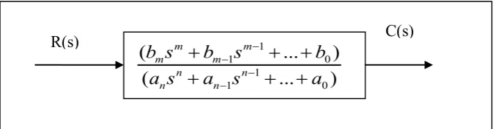
[image:20.595.128.485.511.604.2]The block diagram below shows the transfer function with the left is the
input, the right is the output and inside the block is the system transfer
function. The denominator of the transfer function is identifical to the
characteristic polynomial of the differential equation.
Figure 2.2 : Block diagram of the transfer function
1 1 0 1 1 0(
...
)
(
...
)
m m m m n n n nb s
b s
b
a s
a s
a
2.1
Model Predictive Control (MPC) is an advanced method of process control.
MPC is a form of control in which the current control action is obtained by solving
on-line
, at each sampling instant, a finite horizon open-loop optimal control problem, using
the current state of the plant as the initial state; the optimization yields an optimal
control sequence and the first control in this sequence is applied to the plant[4].
Nowadays, it is being popular among in the industry. MPC has become the primary
form of advanced multivariable control in the process industry and a number of
companies have developed and offered MPC products[5]
Figure 2.3 : Basic Structure of MPC[6]
Figure 2.4 : Basic Concept of Model Predictive Controller[8]
MPC is a controller that uses an identifiable model of a certain process to
predict its future behaviour over an extended prediction horizon and the aim is to minimize
the cost function. The manipulated variable moves is implemented at a sampling instants
over the control horizon is evaluated. The feedback is achieved by implementing the first
move only and then the sequence will be repeated again and this is known as moving
horizon concept [8] Most of the research work done is the application of MPC controller in
specific processes such as gas recovery unit [9], gaseous pilot plant [7], shell and tube heat
exchanger [10] and pasta drying process[11] Large prediction horizon improves nominal
stability of the closed loop but too large of prediction horizon will take long computational
time [7] Advance control strategy such as MPC can lead to energy efficiency. This can
implement by combining the control structures with online process measurements which
can reduce the energy consumption [11].
the performance of the controllers and tuning strategy [8] by comparing the rise time,
percent overshoot and settling time. Moreover, the set point tracking and disturbance
rejection that causes the process to deviate from the desired operating condition can be the
evaluator of the controller performance [8].
2.5
ANALYSIS
In this phase, the performance of the controller can be measured at some criteria
to obtain the optimum control of the process by performance evaluation. To validate the
tuning strategies and further performance assessment, the set point tracking and
disturbance rejection tests will be run [8].
2.5.1
Transient Response
The transient response is defines as the part of total response which
approaches zero as time approaches infinity [3]. Transient response of the
system can be pictured clearly from the step response [12]. For first order
system, it has one pole on the real axis and time constant is the specification of
the transient response that being derived. The time response is the time for the
step response to reach 63% of its final value. It is the reciprocal of the real-axis
pole location and gives an indication of the transient response speed.
2.5.2
Performance Evaluation
The step response performances for MPC controller are evaluated by
observing the rise time, settling time and percentage of overshoot criteria.
Rise time (Tr) is the time taken from the initial set point raise until the
new set point. Long rise time will result in slow response to the controller thus
short rise time is usually required.
Settling time (Ts) is defined as the time for the response to reach the
value of within 98% to 95% from the final value [12]. As for this work, 95%
settling time will be use. Settling time can be related to rise time and decay
ratio.
Overshoot is the maximum amount in which the process variable
exceeds the set point change.
2.5.3
Robustness Tests and tuning validation
It is important to tune the controllers to be robust. The control system is
considered robust if with a certain amount of changes in the process
parameters, the controller can tolerate the changes with stable feedback system
[13]. In this thesis, the robustness test was completed by running a few tests
including Disturbance Rejection, Random Set Point Tracking, White Noise
Input Disturbances and White Noise Plant Disturbances.
For set point changes and set point tracking is to show that the
controller should be able to track the system to operate to any set point
changes. Time taken for the controller to trail the new set point will be
observed.
![Figure 2.3 : Basic Structure of MPC[6]](https://thumb-ap.123doks.com/thumbv2/123dok/574598.68110/21.595.166.480.298.490/figure-basic-structure-of-mpc.webp)
