http://erx.sagepub.com/
http://erx.sagepub.com/content/early/2014/03/06/0193841X13513025
The online version of this article can be found at:
DOI: 10.1177/0193841X13513025
published online 18 March 2014
Eval Rev
Linda Zhao
Richard Berk, Emil Pitkin, Lawrence Brown, Andreas Buja, Edward George and
Experiments
Covariance Adjustments for the Analysis of Randomized Field
Published by:
http://www.sagepublications.com
can be found at:
Evaluation Review
Additional services and information for
http://erx.sagepub.com/cgi/alerts
Email Alerts:
http://erx.sagepub.com/subscriptions
Subscriptions:
http://www.sagepub.com/journalsReprints.nav
Reprints:
http://www.sagepub.com/journalsPermissions.nav
Permissions:
http://erx.sagepub.com/content/early/2014/03/06/0193841X13513025.refs.html
Citations:
What is This?
- Mar 18, 2014
OnlineFirst Version of Record
Covariance
Adjustments for
the Analysis of
Randomized Field
Experiments
Richard Berk
1,2, Emil Pitkin
1,2, Lawrence Brown
1,2,
Andreas Buja
1,2, Edward George
1,2,
and Linda Zhao
1,2Abstract
Background: It has become common practice to analyze randomized experiments using linear regression with covariates. Improved precision of treatment effect estimates is the usual motivation. In a series of important articles, David Freedman showed that this approach can be badly flawed. Recent work by Winston Lin offers partial remedies, but important problems remain. Results: In this article, we address those problems through a refor-mulation of the Neyman causal model. We provide a practical estimator and valid standard errors for the average treatment effect. Proper generalizations to well-defined populations can follow. Conclusion: In most applications, the use of covariates to improve precision is not worth the trouble.
1Department of Statistics, University of Pennsylvania, Philadelphia, PA, USA 2Department of Criminology, University of Pennsylvania, Philadelphia, PA, USA
Corresponding Author:
Richard Berk, Department of Criminology, Department of Statistics, University of Pennsyl-vania, 400 Jon M. Huntsman Hall, 3730 Walnut Street, Philadelphia, PA 19104, USA.
Email: [email protected]
Evaluation Review 1-27
ªThe Author(s) 2014
Keywords
randomized field experiments, covariate adjustments, Neyman causal model.
Introduction
Researchers in the social and biomedical sciences often undertake the analysis of randomized field experiments with a regression model that includes indicator variables for the treatment and covariates thought to increase the precision of estimated treatment effects. The canonical formu-lation is nothing more than a conventional linear regression analysis having as predictors one or more indicator variables for the interventions and one or more covariates thought to be related to the response.
Many popular textbooks recommend this approach (Cox 1958; Kirk 1982; Wu and Hamada 2000). Thus, Wu and Hamada suggest ‘‘When aux-iliary covariates are available, use analysis of covariance and regression analysis to incorporate such information in the comparison of treatments’’ (Wu and Hamada 2000, 84). It may not be surprising, therefore, that results from covariance-adjusted randomized experiments are common in criminal justice research (Maxwell, Davis, and Taylor 2010; Jeong, McGarrell, and Hipple 2012; Koper, Taylor, and Woods 2013; Graziano, Rosenbaum, and Schuck 2013; Asscher et al. 2013). It also may not be surprising that covar-iance adjustments for randomized experiments are often undertaken as part of more complicated analysis procedures, such as hierarchical linear models (Prendergast et al. 2011; James, Vila, and Daratha 2013).
In a very recent article, Lin (2013) examines Freedman’s arguments with the intent of providing improved procedures for practitioners. He replicates Freedman’s overall results and then turns to a conceptual framework that differs substantially from Freedman’s. Within that framework, he is able to guarantee improved precision asymptotically. In addition, his standard errors are unbiased asymptotically so that in large samples, valid confidence intervals and statistical tests can be applied. There remains, however, the need for greater clarity on a number of key points and for more practical estimation procedures.
Lin’s article helps to motivate the approach we take in the pages ahead. We begin with a brief review of the ubiquitous Neyman causal model. It is the approach that Freedman adopts. We then develop an alternative formu-lation that extends the reach of the Neyman causal model, in much the same spirit as Lin’s work. A very practical estimator follows that performs better asymptotically than current competitors. Valid standard errors are also provided. The estimator’s use is illustrated with real data.
Still, Freedman’s advice for practitioners merits serious consideration. Textbook t-tests, perhaps generalized to analysis of variance, work well. Analyses with small samples will often benefit from increased power, but it is precisely in small samples where covariance adjustments can fail badly. With large samples, there will be commonly sufficient precision without introducing covariates into the analysis. Then, the use of covariates needs to be justified in a convincing fashion.
The Neyman Framework
The defining feature of randomized experiments is random assignment of study units. Any conceptual framework for the proper analysis of randomized experiments must be built around random assignment (Neyman 1923).1
There is a set ofnstudy subjects, each of which has apotentialresponse under the treatment condition and a potential response under the control condition. Some number of the subjects nT are assigned at random to the treatment condition with nC ¼ n"nT then assigned to the control
condition. For ease of exposition, we assume one experimental group and one control group.
There is for each subject i an observed response Yi under either the experimental or the control condition (but not both), and an observed set of covariate values xi. The xi are fixed over hypothetical randomizations
important to stress that random assignment is the only source of randomness in the data.2
Statistical Inference
Imagine that all of the study subjects were assigned to the treatment and their responses observed. Imagine that all of the study subjects were assigned to the control condition and their responses observed. Finally, imagine computing the difference between the mean of all the responses under the treatment condition and the mean of all the responses under the control condition. This defines the ‘‘average treatment effect’’ (ATE) that one seeks to estimate. The same basic reasoning can be applied to binary response variables and population proportions. We postpone a consider-ation of binary outcomes until later.
There is no formal role of some larger, finite population that then study subjects are meant to represent. Statistical inference is motivated by an appreciation that the data being analyzed could have been different—the data are but one realization of the random assignment process applied to the study subjects on hand. Hypothetically, there is a very large number of different data realizations that vary solely because thegivenstudy subjects are being assigned at random repeatedly to the experimental and control conditions. It is often convenient to treat the totality of these realizations as the population to which inferences are drawn. Thus, there is no consid-eration of how the study subjects were initially chosen, and no statistical rationale for generalizing the results beyond those study subjects.
An intuitively pleasing plug-in estimate is routinely used: the difference in the data between the mean response of the experimentals and the mean response of the controls. Because of random assignment, this estimate of the ATE is unbiased regardless of the sample size. Arriving at proper statistical tests is not quite so straightforward.
But conventional practice has by and large taken a different path. Researchers commonly favor textbook t-tests or extensions to analysis of variance. The experimental group and control group are at least implicitly treated as random samples from a much larger population, just as in survey research. Sampling is usually done without replacement and all of the rea-lized variables are random, not fixed, variables—this is not the Neyman model. Yet, when the sample is small relative to the population, theory and practice based on the normal distribution generally works well (Freedman, Pisani, and Purves 2007, chapter 27, section 4). That is, the statistical tests violate key elements of Neyman’s formulation, but usually do little inferen-tial damage.
One can also proceed within a linear regression framework. The Neyman framework is implicitly discarded once again, but performance is still reasonable in practice. Thus,
Yi ¼b0þb1Iiþei; ð1Þ
whereiis the subject index,Iiis a 1/0 indicator for which ‘‘1’’ represents the
treatment condition and ‘‘0’’ represents the control condition, and ei is an
unconventional disturbance term.
In Equation 1,eimust be related toIi, the only source of randomness, and
is neither independent and identically distributed nor mean zero. Neverthe-less, we get a ‘‘weak’’ form of orthogonality between Ii and ei because
deviations around the means for the experimentals and controls necessarily sum to zero (Freedman 2006, 4). An ordinary least squares estimate ^b1 is then an unbiased ATE estimate regardless of sample size.3
Conventional regression standard errors can be used for t-tests. The regression estimator assumes the same disturbance variance for the experi-mental outcome and the control outcome. The usualt-test for the difference between means allows for the disturbance variance for the experimentals to differ from the disturbance variance for the controls. Still, conventional regression can work well in practice unless this form of heteroscedasticity is quite extreme.
Equation 1 isnota structural equation model. It is just a convenient com-putational device with which to obtain ATE estimates and standard errors. But because Equation 1 looks like the kind of linear regression used in cau-sal modeling, it is all too easily treated as such. Misunderstandings of this sort have real bite when covariates are introduced, as we will soon see.
methods envision conventional random sampling in which the sample is substantially smaller than the population. Neither is consistent with the Neyman model. But in practice, both are usually satisfactory.
Introducing covariates.It has become common practice to include in Equation 1 one or more covariates to improve the precision of ^b1. For a single covariate,
Yi¼ b0þb1Iiþb2Xiþei; ð2Þ
whereXi is a fixed covariate thought to be related toYi, and all else is the
same as in Equation 1. In particular, one still does not have a conventional regression disturbance term, and Equation 2 is not a structural equation model. Like Equation 1, Equation 2 is merely a computational device.
Researchers often include several covariates, all in service of improved precision in the estimate ofb1, and there can be several different interven-tions, sometimes implemented in a factorial design. One can also find extensions into more complicated regression formulations such as hierarch-ical linear models. There is no need to consider such extensions here. We can proceed more simply with no important loss of generality.4
When a covariate is added to Equation 1, it would seem that the only change is from bivariate linear regression to multivariate linear regression. If Equation 1 is adequate, Equation 2 can only be better. But any actual improvements depend on certain features of the expanded equation.
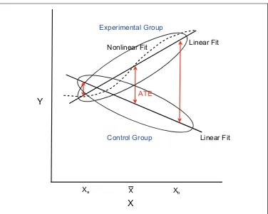
Freedman stresses that Equation 2 must be first-order correct. That is, expectations of the fitted values from Equation 2 over realizations of the data must be the same as the conditional means of the response in the pop-ulation composed of all possible realizations of the data. This means that within the experimental group and within the control group, the response must be related to the covariate in a linear manner, and the slopes of the two lines must be the same. Any treatment effect is manifested in the gap between the two slopes. Figure 1 is an illustration.
When Equation 2 is first-order correct, the desirable properties of Equation 1 carry over, and there is the prospect of improved precision. The constant gap between the two regression lines, represented byb1, is on the average how the response differs between the two groups. One still has an unbiased estimate of the ATE. The usual regression standard errors also can perform reasonably well. But why should Equation 2 be correct?
on hand. As others have pointed out (Heckman and Smith 1995; Berk 2005), without a sensible target population, the rationale for doing rando-mized experiments can be unclear.
The point of doing an experiment is to learn about the impact of interven-tions for some population of theoretical or policy interest. Thinking back to the classic polio experiments, the whole point was to learn from the study subjects how the polio vaccine would work in the population of children around the world. What would happen if they were all vaccinated? What would happen if they were all not vaccinated? Thus, the study subjects were taken to be a representative sample from that population. Clearly, key fea-tures of the Neyman causal model no longer apply. We need another way of thinking about randomized experiments.
Another Formulation
We begin with a set of random variablesZthat have a joint probability dis-tribution with a full-rank covariance matrix and four moments.5With those moments as mathematical abstractions for common descriptive statistics
X Y
ATE
Experimental Group
Control Group
such as means, variances, and covariances, the joint probability distribution can be properly seen as a population from which data could be randomly and independently realized. Alternatively, the population is the set of all potential observations that could be realized from the joint probability distribution. Both definitions are consistent with the material to follow, but the second definition may seem more grounded for many readers.
Using subject–matter information, a researcher designates one of the random variables to be the responseYand one or more other of the random variables as covariates X. There is then a conditional distribution YjX
whose conditional expectations EðYjXÞ constitute the population response surface. No functional forms are imposed and for generality, we allow the functional forms to be nonlinear.
It is important to emphasize that by taking a joint probability distribution as a starting point,YandXare both random variables. Key parameters of the population are, therefore, expected values of various kinds. Standard approaches to probability sampling treat the population variables as fixed (Thompson 2002, section 1.1), so that the usual summary statistics can be population parameters. Our random variable approach leads to significant differences in the statistical theory and notation we use.
For now, we consider only a single covariate. We imagine that all hypothetical study subjects are exposed to the experimental condition. Alternatively, we imagine they are all exposed to the control condition. Under the former, there is for each individual a potential outcome and a value for the covariate. Under the latter, there is likewise a potential out-come and a value for the covariate. Both sets of outout-comes can vary over individuals. For notational clarity, we useTito representYiwhen a subject
i is exposed to the treatment condition andCito representYiwhen a
sub-ject i is exposed to the control condition. Ti and Ci are still potential
responses.
The ATE isdefinedas the difference between the population expectation
E(T) and population expectation E(C). We also want to make use of any association between Y and X. For that, we need to return to the idea of a response surface.
squares, the disturbancesni anduinecessarily have a mean of zero and are
uncorrelated with Xi.
Experimental group Ti ¼ a0þa1Xiþni; ð3Þ
Control group Ci ¼ g0þg1Xiþui: ð4Þ
No claim is made that Equations 3 and 4 result in parallel response surfaces. No claim is made that either can reproduce the actual conditional expecta-tions of the response in the population. The true response surfaces can be substantially nonlinear. The flexibility of this formulation means that Freedman’s concerns about model misspecification no longer apply or, as we show shortly, can be constructively addressed. That is, mean function specification errors do not matter. There can be omitted covariates, for instance.
In the population, the average treatment effect is derived as:
t¼ a0"g0þ ða1"g1Þy; ð5Þ
whereyis the expectation of the covariateX. The value oftis the difference between the intercepts of the two equations, adjusted for the covariate X. Our goal is to estimate the value of t.
Estimation
Consider a realized random sample of study subjects from a population of possible study subjects, all necessarily characterized by the same joint probability distribution. For ease of exposition, suppose that the data are a simple random sample. Subsequently, some of the sampled units are assigned to the treatment condition and the rest are assigned to the control condition. There are now two sources of randomness: the random sampling and the random assignment. This is effectively the same as drawing one random sample from a population to use as the experimental group and another random sample from that population to use as the control group. When the former is exposed to the treatment condition, we get to see T. When the latter is exposed to the control condition, we get to seeC.
To obtain estimates of the ATE, we apply least squares regression to the sample of experimentals consistent with Equation 3 and least squares regression separately to the sample of controls consistent with Equation 4. From these, we obtain estimates ^a0
;^a1;^g0; and ^g1. The estimates can be
Estimates of
y
and the ATE Estimator Properties
Like Freedman and Lin, we rely on asymptotics. Some of the technical details are discussed in the appendix. A far more formal and complete treat-ment can be found in a working paper by Pitkin, Brown, and Berk (2013). We imagine being able to generate a very large number of random samples from the set of potential study subjects, each with a revealed Ti
orCi, andXi. For any given sample, there are three possible ATE estimators
that depend on what is used for the value ofy in Equation 5.
For Lin, the population from which the subjects are drawn is real and finite. The researcher is assumed to know the population mean for the covariate, which can be used as the value ofy. In most social science appli-cations, that mean will not be known.
As an alternative, one might compute for the experimental group regression the fitted value at the mean of its covariate values (i.e., at the mean of the cov-ariate for the experimental group). For the control group regression, one might also compute the fitted value at the mean of its covariate values (i.e., at the mean of the covariate for the control group). But because each set of fitted values must go through the mean of its response and the mean of its covariate values, the estimate of the ATE is no different from the ATE estimate ignoring the covariate. The covariate adjustment changes nothing. One is simply com-paring the mean response for the experimentals to the mean response for the controls. Even if gains in precision are possible, those gains are not achieved.
A preferred approach.Instead of using two different estimates of the covari-ate mean, one for the experimentals and one for the controls, one can use a single estimate for both by pooling the covariate values across the two groups. This makes sense because for both groups, the covariate values are realized from the same covariate distribution in the population.
It is also possible to make good use of a centering strategy. One subtracts the pooled value ofyfrom the covariate values for both the experimentals and controls, and otherwise applies Equations 3 and 4 as usual. Then, the differ-ence betweena0andg0is the ATE estimate. There is no need for Equation 5. Suppose one were to allowyto be any value of the covariate, not just the pooled covariate mean. Because we do not require that the population response surfaces be the same for the experimental group and control group, ATE estimates at other than the pooled mean of the covariate will depend on the two estimated mean functions. These are effectively arbitrary and unlikely to be correct. Expectations of the fitted values are not the same as the conditional means of the response in the population. Consequently, treatment effect estimates are biased asymptotically.
Figure 2, shows population regression lines for the experimentals and controls that differ and are incorrect. The proper ATE estimate is found at the pooled mean of the covariate. If the value of Xb is used instead, the
estimate is incorrect and much larger. If the value ofXais used instead, the
estimate is incorrect, smaller, and with a different sign.
In addition, one or both of the mean functions may be nonlinear. Figure 2 shows with a dashed line a nonlinear mean function for the experimental group. Now that gap between the mean function of the experimental group and the mean function of the control group changes at a rate that is not constant. A proper estimate of the ATE can still be obtained at the pooled mean of the covariate, but not elsewhere.
Precision.Perhaps the major claim by those who favor the use of covariates and linear regression for the analysis of randomized experiments is that the precision of treatment effect estimates will be improved. Consider a varia-tion on our populavaria-tion model.
Ti ¼ a0þa1XiþfiT þxi; ð6Þ
Ci ¼ g0þg1XiþfiC þzi: ð7Þ
In Equation 6,fiT represents for experimental group memberiany
popula-tion disparity between the condipopula-tional expectapopula-tion from the linear least squares regression and the conditional expectation of the response function. In Equation 7,fiC represents for control group memberiany population
group, respectively, between response values and the true conditional means. For the experimental group and control group separately, they are the ‘‘true’’ disturbances around the ‘‘true’’ response surface.
In Equations 3 and 4, the fitting disparities and the true disturbances were combined inni andui. Because Equations 3 and 4 were least squares
regressions, the combined disturbances ni and ui were uncorrelated with
their respective covariate values. One can show that this prevents asympto-tic bias in sample estimates of the ATE. But the unknown fitting disparities affect estimates of the residual variance in a perverse manner (Pitkin, Brown, and Berk 2013).
It can then be shown that the estimated asymptotic standard error for the estimated ATE is
d SEðtÞ ¼
ffiffiffiffiffiffiffiffiffiffiffiffiffiffiffiffiffiffiffiffiffiffiffiffiffiffiffiffiffiffiffiffiffiffiffiffiffiffiffiffiffiffiffiffiffiffiffiffiffiffiffiffiffiffiffiffiffiffiffiffiffiffiffiffiffiffi
d MSET
nT
þMSEd C
nC þ1
2ða^1"^g1Þ 2s^2x
n
s
; ð8Þ
X Y
ATE
Experimental Group
Control Group
X
Xa Xb
Linear Fit
Linear Fit Nonlinear Fit
where subscriptsTandCrefer to the experimental group and control group respectively,ndenotes a number of observations,s2represents a variance, MSE is a regression mean squared error, and a1 and g1 are the regression coefficients associated with the covariate as before. All of the symbols with ‘‘hats’’ are estimates from the sample. TheMSE from each equation can bed separately obtained for the experimentals and controls as part of conventional regression output.
In Equation 8, MSE has two components: the estimated variance ofd the true disturbances around the population response surface and the estimated variance of disparities between the expectation of the condi-tional means from the population linear regression and the actual population conditional means. Their sum constitutes the usual mean squared error of a regression and in practice, the two components can-not be disentangled.7
One can prove that asymptotically,SEdðtÞwill almost always be smaller than the standard error that results when the covariate is excluded (Pitkin, Brown, and Berk 2013). It can be slightly larger if the covariate is unrelated to the response and should not, therefore, have been included in the analy-sis. One gives up a degree of freedom with no compensatory reduction in the residual variance.
More Than One Covariate
Generalization beyond a simple covariate is straightforward. We begin by expanding the number of covariates in the population linear regressions.
Ti¼ a0þa1xi1þ. . .þapXipþfiT þni: ð9Þ
Ci ¼g0þg1xi1þ. . .þgipXpþfiC þui: ð10Þ
The ATE definition must be adjusted accordingly, and the estimator falls in line. Thus,
^
t ¼ ðT!"C!Þ "X!0ða^"^gÞ
: ð11Þ
!
X is a vector of the p covariate means for the experimental group and control group combined.8These may be estimated from the data as described earlier. The values ofa^and^gare vectors of thepestimated regression coeffi-cients (but not the intercepts) for the experimental and control group, respec-tively. As before, if one works with centered covariates, the difference in the interceptsða^
0"^g0Þis the ATE estimate.
d
Equation 12 is the new expression for the estimated standard error of^t, in which all of the previous notation carries over, andP^xis the sample covar-iance matrix of the predictors for the pooled data. As before, the twoMSE’sd can be routinely obtained from their respective regression output. The same holds for all of the arguments in Equation 12. If one does not have access to a programming language such as in R or in STATA, SEdðtÞ can be easily obtained with a pocket calculator.SEdðtÞhas excellent performance asymp-totically (Pitkin, Brown, and Berk 2013).10
Finally, Equations 9 and 10 assume that the included covariates are determined once and for all before the regression analysis begins. There is no model selection. For example, trying various combinations of covari-ates in search of the combination that yields the smallest value forSEdðtÞis ruled out. Just as in any kind of regression analysis, model selection can lead to seriously biased parameter estimates and statistical tests that do not perform properly (Leeb and Po¨tscher 2006; Berk et al. 2010). If the sample size is at least several times larger than the number of prospective covari-ates, it will often make sense to simply include all of them.11
Binary Responses
The mean of a binary variable coded 1 and 0 is a proportion. One might expect, therefore, that our formulation can apply to binary response variables. The ATE becomes the difference in proportions rather than the difference in means.
Perhaps unexpected is that one can proceed with ordinary least squares just as before. The estimate of ATE is asymptotically unbiased, and the sample version of Equations 11 and 12 still apply. However, because of the linear form of regression fit, one can in principle obtain estimates of the pro-portions for the experimentals and controls that are larger than 1.0 or smaller than 0.0. It follows that the difference in the proportions can be less than "1.0 or more than 1.0.
covariate distributions for the experimentals and controls have little or no overlap, and the covariate slopes are very different, it is possible to arrive at ATE estimates larger that 1.0 or smaller than"1.0. Fortunately, because the experimentals and controls are both random samples from the same pop-ulation, this is a highly unlikely occurrence unless the sample size is very small (e.g., <20). Moreover, the ATE standard errors should show that the point estimates are not to be taken very seriously.12
Count Responses
The methods proposed should work adequately for count data. Each count is simply treated as a quantitative response. The ATE is again the difference between conditional means. Our standard errors apply.
Probably the major concern is obtaining fitted values less than 0. Just as with binary data, this should be a very rare occurrence found only in very small samples. And again, the standard errors should convey proper caution.
Working With Convenience Samples
By and large, RCTs are not conducted with random samples. The usual practice is to work with convenience samples. Our approach does not for-mally apply when the units randomly assigned are not a random sample from a larger population.
Nevertheless, under the right circumstances, one may be able to credibly proceed as if the convenience sample is a random sample. One should try to make a convincing argument that treating the data as a random sample is reasonable. That will depend on how the sample was constructed and on the nature of both the intervention and the response.
A Brief Example
Beginning on October 1, 2007, the Philadelphia Department of Probation and Parole (ADPP) launched a randomized experiment to test the impact on recidivism of reducing the resources allocated to low-risk offenders (Berk et al. 2010). Enrollment of low-risk offenders began on that date. At intake, each probationer or parolee was assigned a risk category devel-oped for the ADPP to forecast which offenders were unlikely to be arrested for new crimes while under supervision. Those projected to be low risk were included in the experiment until the target sample size of 1,200 was reached. Enrollment proceeded sequentially.
Although the study subjects were not literally a random sample of parolees and probationers, it is perhaps reasonable to treat the study subjects as a useful approximation of a random sample of low-risk parolees and pro-bationers in Philadelphia for several years before and several years after the study. The number of parolees over that time is well over 200,000 and that was the population to which inferences were to be drawn. There was no evi-dence of short-term secular trends in the mix of probationers or parolees over that interval. There were also no important changes in the State Penal Code or ADPP administrative practices.
Shortly after intake, the equivalent of a coin flip determined the arm of the experiment to which a low-risk offender was assigned. Approximately half were assigned at random to the Department’s regular form of supervi-sion, and the reminder were assigned at random to what one might call ‘‘supervision-lite.’’ For example, mandatory office visits were reduced from once a month to once every 6 months.
The outcome of interest was binary: whether there was a new arrest within the 12-month follow-up period. After a 12-month follow-up, 15% of the control group were rearrested compared to 16%of the experimental group. Using the standard two-sample t-test, the null hypothesis of no difference could not be rejected at anything close to conventional levels. Supervision-lite had virtually no demonstrable impact on recidivism. The weight of the evidence supported a dramatic reduction in supervision for low-risk offenders. As a result, the ADPP reorganized its supervisory resources accordingly.
last two, we included three covariates: the risk score used to identify the low-risk offenders, race, and the age at which a first arrest was recorded.
We included the risk score because it was derived from a large number of predictors related to recidivism and because it had a strong association with rearrest for the full set of offenders. That is, it forecasted well across all types of offenders. We expected a modest association at best for the low-risk subset of offenders. We included race because it was on political grounds excluded from the set of predictors used to construct the risk score and also had a demonstrated association with risk. We included the age vari-able even though it has been incorporated in the risk score because it might have some association with response than had not been captured in the risk score.
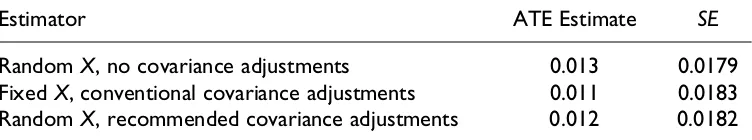
Table 1 shows that all three methods have effectively the same ATE estimate and standard error. One cannot reject the null hypothesis of no dif-ference for any of the estimators. We also estimated the standard error using the nonparametric bootstrap, which like all bootstrap procedures is only jus-tified asymptotically. The estimated standard error is 0.0184, virtually the same as the other standard error estimates.
With the sample size of 1,157, there are effectively no concerns about small-sample bias. Each estimation approach can put its best foot forward. Why do they too all perform so similarly?14 For these data, the multiple correlation between the covariates and the response is essentially zero. The covariance adjustments use up three degrees of freedom with no gain in precision. In retrospect, the lack of association makes sense. The off-enders who were subjects in the experiment had already been selected using almost all of the predictor information available. In short, there was no reason to go beyond the conventional difference in means and a two-sample t-test.
Table 1.Three Estimators for the Binary Response of Rearrest During the ADPP ‘‘Low-Risk’’ Experiment.
Estimator ATE Estimate SE
RandomX, no covariance adjustments 0.013 0.0179 FixedX, conventional covariance adjustments 0.011 0.0183 RandomX, recommended covariance adjustments 0.012 0.0182
Note.ADPP¼Philadelphia Department of Probation and Parole; ATE¼average treatment effect;SE¼standard error.
Although the almost total lack of association between the covariates and the response variable is probably unusual, several other criminal justice experiments we reanalyzed were not dramatically different. None of the relevant multiple correlations were larger than .36. Simulations we have performed indicate that precision is not likely to be meaningfully improved unless the multiple correlation is larger than about .40.
For example, we reanalyzed parts of the Portland (Oregon) Domestic Violence Experiment (Jolin et al. 1996) using data obtained from the Inter-University Consortium for Political and Social Research. The key intervention was the creation of a special police unit devoted to misdemea-nor domestic violence crimes. We considered three postintervention outcomes reported by the victim: counts of the number of times beaten up, threatened, or hit. We worked with a sample size of 396 cases. The high-est multiple correlation with the covariates was for the threat outcome: .36. With no covariates, the estimated ATE was .23, effectively zero with counts that often ranged into the 20s. When covariates were introduced, the esti-mated ATE varied from .29 to .30 depending on the estimator. Over all three estimators, the estimated standard error ranged from .24 to .26. Again, the simple difference in means and the textbook t-test was all that was needed.
Conclusion and Recommendations
Freedman effectively critiques regression analyses of randomized experi-ments in which covariates are introduced. But in our view, there are more fundamental problems. Freedman works from the Neyman formulation that imposes significant constraints on how practitioners can proceed. Because the covariates are treated as fixed, generalizations beyond the data on hand have no formal rationale.
Lin implicitly loosens the ties to the Neyman approach by making use of a real, finite population from which the data can be treated as a random sample. His conclusions are less pessimistic than Freedman’s. However, his proposed estimator will usually not be operational in prac-tice, and its conceptual foundations could benefit from greater clarity and reach.
or wrong functional forms do not compromise the ATE estimates. Our asymptotic standard errors offer greater precision than current alternatives and should work well in large-sample applications. Even in small samples, they can provide some protection against ATE estimates that are likely to be unreasonable. To enjoy these benefits, however, practitioners will require data from a real random sample or be able to make a convincing case that the data on hand can be usefully treated as such.
Still, one has to wonder if any of these covariance-based options are really worth the trouble. Simple differences in means or proportions are unbiased ATE estimates under the Neyman model or under random sam-pling. No asymptotics are required. One also has textbook tests that are valid with random sampling, and which work reasonably well under the Neyman formulation. Possible gains in precision from covariance adjust-ments are in principle most needed with small samples, a setting in which they currently have no formal justification.
Appendix
The combination of random predictors and unknown nonlinear response surfaces raise issues that the Neyman-fixed predictor approach side-steps. Although this is not the appropriate venue for reviewing our underlying mathematics (see Pitkin, Brown, and Berk 2013), many important insights into our approach can be gained through simple visualizations.
Consider a bivariate joint probability distribution composed of random variables Z. The joint distribution has means (called expectations), var-iances, and covariates much like an empirical population composed of fixed variables. Therefore, the joint probability distribution can be properly seen as a legitimate population from which each observation in a sample is ran-domly and independently realized from that distribution. Alternatively and with perhaps fewer abstractions, the population can be conceptualized as all potential study subjects that could be realized from the joint probability distribution.
Using subject–matter information, a researcher designates one of the random variables as a predictor X, and another the random variable as a response Y. Unlike conventional regression formulations, these designa-tions have nothing to do with how the data were generated.
can be called a ‘‘response surface.’’ In less formal language, the response sur-face is the population mean of the response for each value of the predictor. Figure A1 is a two-dimensional plot showing with the dotted line a popula-tion response surface EðYjXÞ.
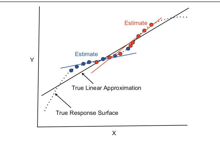
In Figure A1, the solid black line represents the population linear least squares regression of Y on X within the joint probability distribution. As such, it is a linear approximation of the population response surface. The true response surface and its linear approximation usually will be unknown. Each observation in data on hand is taken to be a random realization for the joint probability distribution. A sample is a set of realizations produced independently of one another. The researcher wants to estimate features of the joint probability distribution from the data on hand. There are two approaches that differ by the manner in which the predictor values in the data are viewed.
First, the predictor values can be treated as fixed once they are randomly realized. In other words, one envisions independent repeated realizations of the data, but only for cases with the same set of predictor values in the data on hand. This comports well with common practice, especially in econom-ics. As a formal matter, the sample can be used for generalizations to a joint probability distribution in which only the sample predictor values are found.
X Y
True Response Surface
True Linear Approximation
Estimate
Estimate
For example, if there are no individuals older than 50 in the sample, general-izations of the results to individuals older than 50 have no formal justifica-tion. In short, sample estimates are conditional on the realized predictor values.
Second, the predictor values can be treated as random even when those values are for covariates used in a regression analysis. In other words, one envisions independent repeated realizations of the data, with both the y
values and the x values free to vary as they do in the joint probability dis-tribution. One can formally generalize to the full joint probability distribu-tion, which can be very desirable in policy-driven randomized experiments. The price is a more complicated conceptual framework and a reliance on asymptotic results. But, sample estimates are unconditional with respect to predictor values.
We adopt the second approach. For ease of exposition, suppose for the moment that Y is a deterministic function Xand that there are two sets of realized data from the joint distribution. That is, there are no disturbances contained within the Y values of either sample. The blue circles represent one sample and the red circles represent the other sample. The blue line is the sample least squares line for the blue data, and the red line is the sam-ple least squares line for the red data. As straight lines, neither can capture the true nonlinear response surface. In addition, both lines differ from the true population linear approximation of the true response surface, even though both conditional relationships are deterministic.
Requiring thatYbe a deterministic function ofXis unrealistic. Suppose now that there are conventional disturbances. The dotted line still represents the true conditional expectations of Y given X :EðYjXÞ. But now the red and blue circles are the conditional means of Y given X for the two sets of realized data. Figure A2 is meant to convey how any least squares line from a sample will be a biased estimate of the population linear approximation.
With a nonlinear response surface and the predictor a random variable, any set of realized values will necessarily provide an incomplete picture of the population linear approximation. Biased estimate follows. But the bias disappears asymptotically when the full response surface is revealed— the slope and intercept of a sample regression line are asymptotically unbiased estimates of the slope and intercept of the population linear approximation.
response surfaces are nonlinear but for now, parallel. All vertical distances between the two represent the average difference in their conditional expec-tations and define the ATE. For any value ofX, the ATE is the same.
There are two population linear approximations, one for the experimen-tal group and one for the control group. Because the two response surfaces are parallel, the vertical distance between the lines is also the ATE. As before, the sample least squares lines are biased. But as before, the bias declines with larger sample sizes so that both of the sample slopes and both of the intercepts are asymptotically unbiased. As shown in the figure, how-ever, sample regression lines are not likely to be parallel (hence the bias). It might seem, therefore, that a least squares line for the experimental group and a least squares line for the control group would provide the nec-essary information for a good estimate of the ATE. If the number of obser-vations in the experimental group is the same as the number of obserobser-vations in the control group, and the covariate is mean centered, the difference in the intercepts is an unbiased estimate of the ATE. No asymptotics are required because the bias in the sample regression for the experimental group and the bias in the sample regression for the control group cancel out. Moreover, if the sample sizes are different but known, unbiased estimates may be obtained by computing the correspondingly reweighted average of the two intercepts.
X Y
True Response Surfaces
True Linear Approximations
Estimate for controls
Estimate for Experimentals
ATE
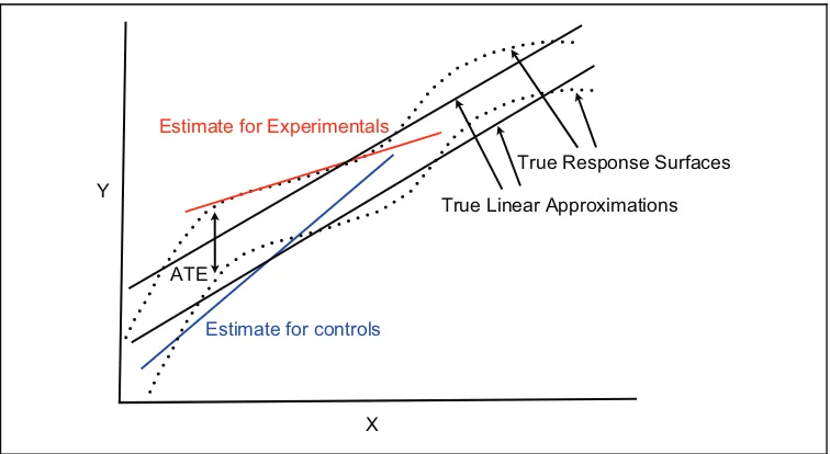
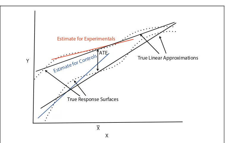
In practice, it will be unusual for a researcher to have parallel true response surfaces for the experimental group and the control group. In practice, more-over, the nature of the true response surfaces will be unknown. Prudence dic-tates, therefore, allowance for true response surfaces that are not parallel.
Figure A3 provides an example. Because the true response surfaces are not parallel, the distance between them is not constant. The same applies to the true linear approximations. Yet, as population least squares lines, both linear approximations must pass through their respective means for the response Y and the mean of the covariate X. It follows that the difference between the linear approximations at the expectation of the covariate defines the population ATE.
Finally, because the sample least squares lines are asymptotically unbiased estimates of their population linear approximations, the distance between the sample least squares line for the experimental group and the sample least squares line for the control group computed at the mean of the covariate is an asymptotically unbiased estimate of the population ATE. These results generalize to situations in which there is more than one covariate.
In practice, a good way to proceed in large samples is to center each cov-ariate on its pooled mean for the experimental and control groups and use
X Y
True Response Surfaces
True Linear Approximations
Estimate for Controls
Estimate for Experimentals
ATE
X
the difference between the intercepts of the two sample least squares lines as the ATE estimate. The expression we provided for the standard error will then allow proper statistical tests and confidence intervals.
Declaration of Conflicting Interests
The author(s) declared no potential conflicts of interest with respect to the research, authorship, and/or publication of this article.
Funding
The author(s) received no financial support for the research, authorship, and/or pub-lication of this article.
Notes
1. The Neyman framework is often called the Neyman–Rubin model because of important extensions and enrichments introduced by Donald Rubin (Holland 1986). The Neyman–Rubin model dominates current thinking about the analy-sis of randomized experiments and quasi experiments (Rosenbaum 2009). But for our purposes, Neyman’s foundational work is what’s relevant.
2. Despite common practice, covariates cannot be ‘‘mediators’’ under the Neyman model. Mediators are variables that can be altered by the intervention that, in turn, impact the response. They depend necessarily on the intervention assigned. In contrast, Neyman covariates are measured before an experimental intervention or if not, are on theoretical grounds treated as causally unaffected. The study of mediator variables requires a very different formulation within structural equation modeling traditions (Wu and Zumbo 2008). The Neyman model no longer applies.
3. One necessarily assumes there is no systematic measurement error in the response and no measurement error of any kind in the treatment indicator. These requirements would be no less essential were one analyzing an experiment
using a conventionalt-test on the difference between means.
4. Stratifying by covariates can also improve precision (Miratrix, Sekhon, and Yu 2013). But the approach differs from regression and is beyond the scope of this article. See Pitkin, Brown, and Berk (2013) for a proper treatment. There are a variety of other matching procedures, but in general covariance adjustments are more effective if the goal is increased precision.
5. These requirements of the joint probability distribution rarely matter in practice. 6. An approach taken by Imbens and Wooldridge (2009) has many parallels, but
they assume that the model is correct.
7. Here, one only needs to estimate the sum of the disturbance variance and the
8. As pointed out earlier, if the separate covariate means for the experimental group and the control group are computed from the data and used, one is returned to the ‘‘naive’’ estimator from no gains in precision are possible. 9. The centering is done with covariate means computed from the pooled data. 10. If requested, the authors can provide code in R for estimates of the proper
stan-dard errors.
11. As already noted, the covariates are included solely to improve precision. They have no subject–matter role in part because we allow the regression equations to be wrong. One happy result is that high correlations between the covariates are of no concern unless they are so high that the usual least squares calculations cannot be undertaken.
12. We have just begun to explore whether our formulation can be properly applied to the full generalized linear model and in particular, binomial regression. The technical issues are challenging.
13. A less powerful generalization approach employs stratification. One subsets the data into groups with similar values for the covariate. For each of these groups, a separate analysis is undertaken. The approach loses power because the orig-inal sample is spread across strata. And with smaller samples, asymptotic prop-erties may not be very comforting. Details can be found in Pitkin, Brown, and Berk (2013).
14. All three estimated standard errors are from a single data set. Size comparisons across the estimated standard errors convey little about their average relative performance. Moreover, there is an apples and oranges problem because fixed
X approaches and random X approaches are addressing somewhat different
sources of uncertainty.
References
Asscher, J. L., M. Dekovic´, W. A. Manders, P. H. van der Laan, and P. J. M. Prins. 2013. ‘‘A Randomized Controlled Trial of the Effectiveness of Multisystemic Therapy in the Netherlands: Post-treatment Changes and Moderator Effects.’’
Journal of Experimental Criminology9:169–212.
Berk, R. A. 2005. ‘‘Randomized Experiments as the Bronze Standard.’’Journal of
Experimental Criminology1:417–33.
Berk, R. A., G. Barnes, L. Ahlman, and E. Kurtz. 2010. ‘‘When Second Best is Good Enough: A Comparison between a True Experiment and a Regression
Discontinuity Quasi-experiment.’’ Journal of Experimental Criminology 6:
191–208.
Cox, D. R. 1958.Planning of Experiments. New York: John Wiley.
Fisher, R. A. 1971. The Design of Experiments. 9th ed. London, England: Hafner
Freedman, D. A. 2006. ‘‘Statistical Models of Causation: What Inferential Leverage
Do They Provide?’’ Evaluation Review 30:691–713.
Freedman, D. A. 2008a. ‘‘On Regression Adjustments to Experimental Data.’’
Advances in Applied Mathematics 40:180–193.
Freedman, D. A. 2008b. ‘‘On Regression Adjustments in Experiments with Several
Treatments.’’ Annals of Applied Statistics2:176–96.
Freedman, D. A., R. Pisani, and R. Purves. 2007. Statistics. 4th ed. New York:
Norton.
Graziano, L. M., D. P. Rosenbaum, and A. M. Schuck. 2013. ‘‘Building Group Capacity for Problem Solving and Police-community Partnerships through Survey Feedback and Training: A Randomized Control Trial with Chicago’s
Community Policing Program.’’ Journal of Experimental Criminology.
Springer Online, January.
Heckman, J. J., and J. A. Smith. 1995. ‘‘Assessing the Case for Randomized Social
Experiments.’’Journal of Economic Perspectives9:85–110.
Holland, P. W. 1986. ‘‘Statistics and Causal Inference.’’ Journal of the American
Statistical Association81:945–60.
Imbens, G. W., and J. M. Wooldridge. 2009. ‘‘Recent Development in the
Econometrics of Program Evaluation.’’Journal of Economic Literature47:5–86.
James, L., B. Vila, and K. Daratha. 2013. ‘‘Results from Experimental Trials Testing Participant Resposes to White, Hispanic, and Black Suspects in High Fidelity
Deadly Force Judgement and Decision-making Simulations.’’ Journal of
Experimental Criminology9:189–212.
Jeong, S., E. F. McGarrell, and N. K. Hipple. 2012. ‘‘Long-term Impact of Family Group Conferences on Re-offending: The Indianapolis Restorative Justice
Experiment.’’ Journal of Experimental Criminology8:369–85.
Jolin, A., R. Fountain, W. Feyerherm, and S. Friedman. 1996. Portland [Oregon]
Domestic Violence Experiment, 1996 – 1997. ICPSR 3353, Ann Arbor, MI.
Kirk, R. W. 1982.Experimental Design. 2nd ed. Belmont, CA: Brooks/Cole.
Koper, C. S., B. G. Taylor, and D. J. Woods. 2013. ‘‘A Randomized Test of Initial and Residual Deterrence from Directed Patrols and Use of License Plate Readers
at Crime Hot Spots.’’Journal of Experimental Criminology9:213–44.
Leeb, H., and B. M. Po¨tscher. 2006. ‘‘Can One Estimate the Conditional
Distribution of Post-model-selection Estimators?’’ The Annals of Statistics 34:
2554–91.
Lin, W. 2013. ‘‘Agnostic Notes on Regression Adjustments to Experimental Data:
Reexamining Freedman’s Critique.’’Annals of Applied Statistics 7:295–318.
Maxwell, C. D., R. C. Davis, and B. G. Taylor. 2010. ‘‘The Impact of Length of Domestic Violence Treatment on Patterns of Subsequent Intimate Partner
Miratrix, L. W., J. S. Sekhon, and B. Yu. 2013. ‘‘Adjusting Treatment Effect
Estimates by Post-stratification in Randomized Experiments.’’ Journal of the
Royal Statistical Society, Series B75:369–96.
Neyman, J. 1923. ‘‘On The Application of Probability Theory to Agricultural
Experiments.’’ In Statistical Science, translated and edited by D. M.
Dabrowska and T. P. Speed (1990), 463–80 (with discussion).
Pitkin, E., L. Brown, and R. A. Berk. 2013. Improving Precision in Estimating
Average Treatment Effects. Working Paper. Philadelphia: Department of Statistics, University of Pennsylvania.
Prendergast, M., L. Frisman, J. Y. Sacks, M. Staton-Tindall, L. Greenwell, H. J. Lin, and J. Catier. 2011. ‘‘A Multisite, Randomized Study of Strength-based Case
Management with Substance-abusing Parolees.’’ Journal of Experimental
Criminology 7:225–53.
Rice, J. A. 2007.Mathematical Statistics and Data Analysis. 3rd ed. Belmont, CA:
Brooks/Cole.
Rosenbaum, P. R. 2009.Design of Observational Studies. New York: Springer.
Thompson, S. K. 2002. Sampling. 2nd ed. New York: John Wiley.
Wu, C. F. J, and M. Hamada. 2000. Experiments: Planning, Analysis, and
Parameter Design Optimization. New York: John Wiley.
Wu, A. D., and B. D. Zumbo. 2008. ‘‘Understanding and Using Mediators and
Moderators.’’Social Indicators Research87:367–92.
Author Biographies
Richard Berkis a professor in the Department of Criminology and the Department of Statistics at the University of Pennsylvania.
Emil Pitkinis a graduate student in the Department of Statistics at the University of Pennsylvania.
Lawrence Brownis a professor in the Department of Statistics at the University of Pennsylvania.
Andreas Buja is a professor in the Department of Statistics at the University of Pennsylvania.
Edward Georgeis a professor in the Department of Statistics at the University of Pennsylvania.