A Camera Self-Calibration Method Based on Plane Lattice and Orthogonality

DOI: _{10.12928/TELKOMNIKA.v11i4.1446  767}

A Camera Self-Calibration Method Based on Plane

Lattice and Orthogonality

Yue Zhao*, Jianchong Lei

School of Mathematics and Statistics, Yunnan University Cuihu North Road 2#, Kunming, 650091, China

*Corresponding author, e-mail: zhao6685@yeah.net, cvbertie@126.com

Abstrak

Kalibrasi menggunakan garis orthogonal adalah salah satu pendekatan dasar kalibrasi kamera, tetapi ini membutuhkan garis orthogonal terdeteksi secara akurat, yang menyebabkan peningkatan galat. Makalah ini mengusulkan teknik baru kalibrasi-sendiri kamera menggunakan kisi-kisi datar dan garis orthogonal virtual. Hubungan analitis ketat antara koordinat titik fitur kisi-kisi datar, koordinat titik citra yang sesuai, parameter intrinsik, pose relatif diinduksi sesuai dengan matriks homograpi dari proyeksi pusat. Biarkan kemiringan non-paralel dan garis virtual non-ortogonal pada bidang kisi, dan kemiringan garis orthonormal dapat dihitung. Dalam setidaknya tiga citra yang diambil , titik hilang dapat diselesaikan dalam dua kelompok arah orthogonal dengan menggunakan matriks homograpi, sehingga parameter intrinsik kamera yang linear dapt diketahui. Metode ini memiliki prinsip sederhana dan pembuatan pola yang baik, dan tidak melibatkan pencocokan citra, selain tidak memiliki persyaratan mengenai gerakan kamera. Eksperimen secara simulasi dan data real menunjukkan bahwa algoritma ini adalah layak, dan memberikan akurasi yang lebih tinggi dan kokoh.

Kata kunci: kamera kalibrasi-sendiri, parameter intrinsik, titik lenyap, garis virtual

Abstract

The calibration using orthogonal line is one of the basic approaches of camera calibration, but it requires the orthogonal line be accurately detected, which makes results of error increases. This paper propose a novel camera self-calibration technique using plane lattices and virtual orthogonal line. The rigorous analytical relations among the feature point coordinates of the plane lattice, the corresponding image point coordinate, intrinsic parameters, relative pose are induced according to homography matrix of the central projection. Let a slope of non-parallel and non-orthogonal virtual line in the lattice plane, and the slope of its orthonormal line can be calculated. In at least three photographs taken, vanishing points can be solved in two groups of orthogonal directions by using the homography matrix, so the camera intrinsic parameters are linearly figured out. This method has both simple principle and convenient pattern manufacture, and does not involve image matching, besides having no requirement concerning camera motion. Simulation experiments and real data show that this algorithm is feasible, and provides a higher accuracy and robustness.

Keywords: camera self-calibration, intrinsic parameter, vanishing point, virtual line

1. Introduction

In computer vision, it has an important significance to the investigation of camera calibration, which is the premise and foundation for obtaining three-dimensional (3D) information, and an important part of the binocular visual field. Accurate Calibration of the camera intrinsic parameters can not only directly improve measurement precision but establishes nice base for further realizing stereo image matching and 3D reconstruction. Meanwhile, real-time of calibration can meet the needs of industry machine vision such as spatial query, navigation etc.

is a major focal point of research in the field of computer vision [3-11]. However, the calibration methods which not use geometric data in scene are nonlinear, complicated and poor robustness. Zhang [12] presented a simple and flexible self-calibration method, which utilize a pinpoint lattice template instead of a traditional calibration object. According to the mutual movement between the template and a camera, photographs of the template are taken from more than three different orientations, so the camera intrinsic parameters can be linearly solved by computing the homography matrix between the template and its image. On the basis of Zhang’s method [12], Meng et al. [13] put forward a kind of self-calibration method which used a circle and several lines passing through the center of the circle as a planar pattern to determine the camera intrinsic parameters according to the image of circular points. The self-calibration method based on circular points is first put forward. From then on, a number of calibration methods are proposed on the basis of Zhang [12] and Meng et al.[13]. Wu FC et al. [14] proposed a linear method to determine the camera intrinsic parameters by rectangle. With the deficiency of accurate location for lattice pattern in Zhang’s method [12], Li XJ et al. [15] proposed a camera self-calibration method based on planar similar figure. Wang GH et al. [16] proposed a self-calibration method based on Kruppa equation of checkerboard. In addition, in recent years, some self-calibration methods based on circular points or vanishing point have emerged [17-20]. Meanwhile, many calibration methods of panoramic camera have appeared by using checkerboard pattern [21-22].

Considering that line belongs to one of the basic geometric elements, which is common and easy to detect, so a camera can be calibrated by using virtual orthogonal lines after homography matrix. Taking into account the straight line is one of the basic geometric, common and easy to detect. So in this work, we use virtual orthogonal lines to calibrate after obtain the homography. In contrast with other calibration methods, this approach only needs to establish the homography matrix between world coordinate system (WCS) and image coordinate system. Based on the estimation of the homography matrix, vanishing points can be gotten in two mutually perpendicular directions, so the camera intrinsic parameters can be solved from three images.

2. Camera Model

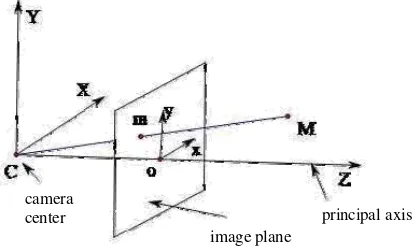
In this study, we use the pinhole camera model which is the simplified model of geometry relation in optical imaging system (see Figure 1).

Figure 1. Pinhole camera model

On the basis of imaging principles of the coordinates of object points in three-dimensional (3D) space and their corresponding points in image plane, a 2D point m and a 3D point M are denoted as ( , )x yT and ( , , )X Y Z T , respectively, and their homogeneous point coordinates are denoted as m ( , , )x y t T and M ( , , , )X Y Z t T , respectively, where t is the homogeneous term, and usually t1. When _, it corresponds to the element on a plane at infinity. The Euclid space which is supplemented with the infinite far element is called an extended Euclid space [8].

principal axis image plane

Under pinhole camera model, a space point ( , , ,1)T

M  X Y Z is projected to its image pointm ( , ,1)x y T . Based on the principle of perspective projection transformation, their relationship is

mPM (1)

where  is an arbitrary scale factor, P is called the projection matrix which can be further broken down into _P_{K R}



_t



with the camera extrinsic parameters

 

R t, . Here, R is a 33 rotation matrix and

t

is a 31 translation vector, which determine the position of WCS with respect to camera coordinate system (CCS), and K is called the camera intrinsic matrix, which

is given by

0

0 0

0 0 1

u

v

f s u

K f v

 

 

  

 

 

, with the coordinates ( ,u v_{0 0})of the principal point, the scale factors

u

f , f_v in image u, v axes, and the parameter s _{describing the skewness of the two image} axes.

3. Estimating the Homography

Without loss of generality, we assume a lattice plane lies on plane XOY (Z0) of WCS. Any point ( , , 0,1)X Y on the lattice plane is transformed from the WCS into the CCS. Then, from (1), it is projected by:



_{1 2 3}





_{1 2}



0

1 1

1

X

X X

Y

m K r r r t K r r t Y H Y



 

   

 

   

 

  _{ } _{ }

 

   

     

 

(2)

where H is the homography matrix between the lattice plane and its image,

r

_i is the

i

thcolumn of the rotation matrix

R

.

Let H be

11 12 13

21 22 23

31 32 33

H H H

H H H

H H H

 

 

 

 

 

.A pair of corresponding points are M



X Y, ,1



 m



x y, ,1



,

and denoted as



11 12 13 21 22 23 31 32 33



T

h H H H H H H H H H . Hence, formally, we have

 

0

0 0

T T T

H T T T

M xM

M M h

M yM

  

   



  (3)

where





4

, , ,

M  X Y x y R is the four-dimensional(4D) vector of nonhomogeneous coordinates including a space point and its corresponding image point, called the measuring spacious point. In fact, the third component of 3D vectorM HM is a linear combination of the first two components, so M_H

 

M is the first two components of M HM . The homography matrix H can be regarded as the intersection set of two quadric surfaces in 4D space, so it is given by:



4

 



0

H H

Suppose



Mj



Xj Yj 1



mj



xj yj 1 ,



j 1, 2, ,n



 

     is a set ofmeasurement

corresponding points from the homography matrix, so a set of



M j



Xj Yj xj yj



T,j1, 2,n



can be gotten according to more pairs of measurement

points. Using a measurement matrix from the set, the homography matrix H can be obtained by solving the following minimization problem:

 

 

2 ,

1

min

0, 1, 2,

j

n

j j

H M j

H j

M M

subject to M M j n

 

 _{ }

 

 _{  }











(5)

4. Solving Camera Intrinsic Parameters

Proposition 1: Assume there is a pair of orthogonal lines on the lattice plane, their points at infinity are denoted as V_1,V_2, and their image point are denoted as v v₁, ₂, so have

1 2 0

v wv  , where _wK_K1_.

Proof: According camera imaging principle, it can be represented as

_{1 1}v K R



T V



_1,_{2 2}v K R



T V



_2 (6)

Rearranging the above equation, we have

1





1





1 1 1 2 2 2

K v  R T V_，K v  R T V_ (7)

Two lines through the infinity points V₁,V₂ are mutually, so the equation is given by

₁T T _{2 1 1}T



 

T ₂



_{2 1 2 1}T



 

T



_{2 1 2 1}T ₂ 0

v K K v V_ R T  R T V_  V_ R T R T V_  V V_{ }  (8)

Let 1

K K

_   _{, therefore, the above equation may be written as}

v

₁



v

₂



0

(9) Image coordinates of arbitrary point can be gotten on a pattern by homography matrix. The point at infinity corresponding to arbitrary line on a plane lies on the plane. If known any point coordinates at infinity, its image coordinates can be obtain, namely the vanishing point coordinates.

Proposition 2: If known arbitrary two either non-parallel or non-orthogonal virtual linear slopes, the five camera intrinsic parameters can be determined with at least three images.

Proof: If let a slope of virtual line on the planar pattern be

k

, the homogeneous coordinates of one point at infinity can be expressed as



1, , 0

k



in the line direction, and the homogeneous coordinates of another point at infinity can be expressed



1, -1

k

, 0



in its orthogonal direction. When given slops of arbitrary two neither parallel nor orthogonal lines, the two lines and the points at infinity of their orthogonal lines can be gotten. The vanishing points corresponding to the two lines can be obtained by the perspective projection transformation. That is

1

1 0

u

v H k



   

  _  

   

   

   

2n constraint equations as (9) can be established with n images

0

T

i j

v v 

where

v

_i ,

v

_j are the vanishing points of two virtual lines in two orthogonal directions.

Let

1 2 3

2 4 5

3 5 6

  



  

  









 











, we can obtain

1 2 1 2 1 1 2 2 1 2 3 1 2 4 1 2 5 6

3 4 3 4 3 3 4 2 3 4 3 3 4 4 3 4 5 6

1 2 3 4 5 6

( ) ( ) ( ) 0

( ) ( ) ( ) 0

( ) ( ) ( ) 0

i j j i i j i j i j i j

u u u v u v u u v v v v

u u u v u v u u v v v v

u u u v u v u u v v v v

                             _{        }                 (11)

Let f 



 _{1 2}    _{3 4 5 6}



T,

1 2 2 1 1 2 1 2 1 2 1 2

3 4 4 3 3 4 3 4 3 4 3 4

1 1

1

i j j i i j i j i j i j

u u u v u v u u v v v v

u u u v u v u u v v v v

A

u u u v u v u u v v v v

     _{  }            ,

Equation (11) becomesAf 0. A linear solution of f is gotten by using the least square method to linearly solve, and  can be obtained. The five camera parameters are determined by Cholesky decomposition of .

We use the established propositions to derive the following algorithm.

Step 1: Make a lattice plane as a template, and take at least three pictures at different azimuths.

Step 2: Use Harris corner detection to get the coordinates of each point on the lattice pattern, and estimate the homography matrix H between the template and its image.

Step 3: Suppose the slopes k k1, 2 _{of two neither parallel nor orthogonal virtual lines on lattice}

plane, and then calculate coordinates of the vanishing point in two orthogonal directions according to (10).

Step 4: Establish the constraint equation according to (9) to obtain through solving (11). Step 5: Determine the five camera intrinsic parameters by Cholesky decomposition of .

5. Experiments

5.1. Simulation results

In simulation experiments, the planar chessboard as a lattice template, the camera intrinsic parameters were set at fu2000, fv 2000, s0.2, u0 800, v0650. The image

resolution is 1480×1240. The checker pattern contains 9×7=63 corner points, and its size of the pattern is 29.7cm×21cm. The extrinsic parameters are as follows:



1 1



0.9393 0.3052 0.1564 7.4965 0.3285 0.9318 0.1545 3.6398 0.0986 0.1965 0.9755 18.7231

R T      _   _     

,



_{2 2}



0.9393 0.3052 0.1564 0.8981 0.1626 0.7978 0.5805 3.6509 0.3020 0.5198 0.7991 14.6923

R T        _   _      ,



3 3



0.7071 0 0.7071 3.5355 0.2185 0.9511 0.2185 5.7457 0.6725 0.3090 0.6725 24.1555

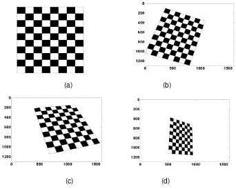
In addition, suppose slopes of two either non-parallel or non-orthogonal virtual lines in lattices plane are k₁  0.25 and k₂0.125, respectively. The chessboard and its images are as follows (see Figure 2).

(a) (b)

(c) (d)

Figure 2. (a) the planar chessboard in space. (b), (c), (d) three images under different orientations

Firstly, estimating the homography matrix and solving the vanishing points of the virtual lines according (10), so establish the constraint equations from (9) to solve linearly 

-10

1975.349173 -0.197527 -1580150.905232

10 -0.197527 1975.349187 -1283818.971818

-1580150.905232 -1283818.971818 1



 

 

 _{  }

 

 

Finally, obtain the five camera intrinsic parameters K can be obtained through Cholesky decomposition of

2000.000008 0.199992 799.999979

0 2000.000011 650.00011

0 0 1

K

 

 

  

 

 

3.2. Real data

The camera to be calibrated is a CCD camera. The image resolution is 320×240. The planar pattern contains 9×7=63 corner points. It was printed with a high-quality printer. Three images of the pattern under different orientations were taken, as shown in Figure 4.

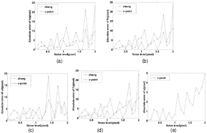
We applied our and Zhang’s calibration algorithm to the three images. The results are shown in Table 1 (the skew factor

s



0

in Zhang’s method).

(a) (b)

[image:7.595.91.509.173.442.2]

(c) (d) (e)

Figure 3. The experimental results of proposed method’s compare with Zhang’s method. (a), (b), (c), (d) the error comparison of the camera intrinsic parameters fu,f u vv, ₀, ₀of this paper’s

method and Zhang’s method. (e) Since let the skew factors0in Zhang’s method, the error of the camera intrinsic parameter s is shown by this paper’s method.

[image:7.595.118.482.527.630.2]

(a) (b) (c)

Figure 4. Three checkerboard images (a), (b), (c) were taken under different orientations

Table 1. Calibrating camera intrinsic parameters with two different methods

All within the

parameters fu fv u0 v0 s

[image:7.595.112.488.705.745.2]

6. Conclusion

In this paper, we presented a novel approach of camera calibration. First, we estimated the homography between the planar pattern and its image. Then, supposed the slopes of two either non-parallel or non-orthogonal virtual lines in lattice plane, used the homography matrix to compute the vanishing points in the directions of two groups of orthogonal lines, and solved the camera intrinsic parameters by vanishing points. the results of simulation and real data showed that this algorithm was feasible and available, and had a certain precision and robustness.

Acknowledgments

This research was supported by the Natural Foundation of Yunnan Province, China (2011FB017).

References

[1] Hartley RI. Estimation of relative camera positions for uncalibrated cameras. In: Proceedings of the European Conference on Computer Vision. 1992; 1: 579-587.

[2] Maybank SJ, Faugeras OD. A theory of self-calibration of a moving camera. The International Journal of Computer Vision. 1992; 8(2): 123-151.

[3] Sturm PF, Maybank SJ. On plane-based camera calibration: A general algorithm, singularities, applications. In: Proceedings of the IEEE Conference on Computer Vision and Pattern Recognition. 1999; 1: 432-437.

[4] Tsai RY. An efficient and accurate camera calibration technique for 3D machine vision. Proc. IEEE Computer Vision and Pattern Recognition Conference. 1986; 1: 364-374.

[5] Zhang Z. Camera calibration with one-dimensional objects. In: Proceedings of 7th European Conference on Computer Vision LNCS 2353. 2002; 1: 161-174.

[6] Hou T, Niu H, Fan D. Speed control for high-speed railway on multi-mode intelligent control and feature recognition. Indonesian Journal of Electrical Engineering. 2012; 10(8): 2068-2074.

[7] Xu ZY, LI Wb, Wang Yun, Luo C, Gao SY, Cao DD. Trinocular calibration method based on binocular calibration. Indonesian Journal of Electrical Engineering. 2012; 10(6): 1439-1444.

[8] Hartley R, Zisserman A. Multiple view geometry in computer vision. Cambridge: University Press. 2000.

[9] Li H, Wu FC, Hu ZY. A novel linear camera self-calibration technique. Chinese Journal of Computers. 2000; 23(11): 1121-1129.

[10] Lei C, Wu FC, Hu ZY. Kruppa equation and camera self-calibration. Chinese Journal of Automation. 2001; 27(5): 621-630.

[11] Wu FC, Li H, Hu ZY. A study on active vision based camera self-calibration. Chinese Journal of Automation. 2001; 27(6): 736-746.

[12] Zhang Z. A flexible new technique for camera calibration. IEEE Transaction on Pattern Analysis and Machine Intelligence. 2000; 22(11): 1330-1334.

[13] Meng XQ, Li H, Hu ZY. A new easy camera calibration technique based on circular points. In: Proceedings of the British Machine Vision Conference. 2000; 1: 496-501.

[14] Wu FC, WANG GH, Hu ZY. A linear approach for determining intrinsic parameters and pose of cameras from rectangles. Journal of software, 2003; 14(2): 703-712.

[15] Li XJ, Zhu HJ, Wu F. Camera calibration based on coplanar similar geometrical entities. PR&AI. 2004; 17(4): 457-461.

[16] Wang G, Jonathan Wu QM, Zhang W. Kruppa equation based camera calibration from homography induced by remote plane. Pattern Recognition Letters. 2008; 29(16): 2137-2144.

[17] Wang H, Zhao Y. A new planar circle-based approach for camera self-calibration. Journal of Computational Information Systems. 2010; 6(9): 2877-2883

[18] Zhao Y, Wang H. Conic and circular points based camera linear calibration. Journal of Information and Coputational Science. 2010; 7(12): 2478-2485.

[19] Zhao Y, Wang H, Wang XF. A conic-based approach for camera linear self-calibration. Journal of Information and Computational Science. 2010; 7(10): 1959-1966.

[20] Wang H, Zhao Y, Li J. Innovation experiment based on circular points and Laguerre theorem in computer vision. In Proceedings of 2nd International Conference on Education Technology and Computer. 2010; 1: 25-28.

[21] Duan HX, Wu YH. A calibration method for paracatadioptric camera from sphere images. Pattern Recognition Letters. 2012; 33(6): 677-684.