Two Dimention Numerical Reconstruction of Electrical Impedance Tomography using Tikhonov Regularization Algorithms with a-posteriori parameter choice rule

(1)

2-D Numerical Reconstruction of Electrical

Impedance Tomography using Tikhonov

Regularization Algorithms with a-posteriori

parameter choice rule.

∗

A.D. Garnadia,†_{& D. Kurniadi}b

a

Department of Mathematics, Institut Pertanian Bogor,

Jl Meranti, Kampus Darmaga, Bogor 16680,

Indonesia

b

Department of Engineering Physics, Institut Teknologi Bandung,

Jl Ganesha, Bandung 40132,

Indonesia

7-8 December 2005

Abstract

Electrical Impedance Tomography, as an Inverse Problem, is calculation of the resistivity distribution due to given boundary potential and current density distribution. Most of the inverse problem are ill-posed, since the measurement data are limited and imperfect. This paper describes a regularization technique for solving the ill-posed problem appeared in the inverse EIT. In this regularization technique, a smoothing function with a regularization parameter, is penalizing the objective function in order to obtain a regularized resistivity update equation. The regularization parameter can be chosen from a-posteriori information. We made comparison of 3 methods, the first method can be thought of as a discrepancy principle, where we select an initial value of the regularization parameter by trial and error technique. The second and third methods are methods adopted from Linear ill-posed prob-lem, with a posteriori information characters. We presents numerically the reconstruction using artificially generated data.

Keywords: Inverse Problems; Nonlinear ill-posed; Tikhonov Regularization ; Reconstruction Algorithms; a-posteriori parameter.

∗_{This work fully supported by Hibah Bersaing XIII 2005-2007 Project.} _{(Contract no}

026/SPPP/PP-PM/DP3M/IV/2005).

†_{Corresponding author. E-mail: adg661@yahoo.com}

(2)

1 Introduction

Electrical Impedance Tomography (EIT) is a computerized tomographic imaging technique which is able to reconstruct an image of the dis-tribution of electrical impedance such as resis-tivity from a knowledge of the boundary volt-age and current on the object. EIT offers a pos-sibility of realizing a low cost and safe imaging system, because it uses non-ionizing radiation and requires relatively simple hardware. Some promising fields of this technique are biomedi-cal engineering, geophysics, non-destructive test, industrial process, humanitarian demining etc. The problem of image reconstruction in EIT is broken into a forward and inverse problem. The forward problem involves finding the po-tential distribution given the resistivity distri-bution and certain boundary condition. The inverse problem calculates the resistivity dis-tribution given measured potential an current density distribution. In this study, we employ the Finite Element Method (FEM) to solve the forward problem, and (Tikhonov Regulariza-tion) method to find the inverse solution where it minimizes, iteratively, an objective function to obtain the update resistivity distribution equa-tion.

Almost all of the inverse problem are ill-posed. In this case, the matrix to be inverted in the equation for calculating the update resistivity distribution is ill-conditioned. This leads to so-lution of that equation may not exist, or al-though a solution does exist, it does not stable. We adopt the well-known Tikhonov regulariza-tion technique to solve the ill-posed problem. We introduce a stabilizing or a smoothing func-tion with a regularizafunc-tion parameter to the ob-jective function, then by minimizing the value of the objective function we will obtain a reg-ularized resistivity update equation.

This study can be seen as a continuation of [2] in the context of [7], it is worth to notes that [3] studied Tikhonov Regularization to solve EIT problem studying coefficients mathemat-ical regularity. In [8] and [9] which is forbear of [7], they did not address in details on how to choose the regularization parameter.

2 Reconstruction Technique

Calculation of Resistivity Distribution

To calculate the internal resistivity distribution of an object from boundary potential and cur-rent data, we evaluate iteratively an objective function that describes the error between the voltage response of the real object and that of the model. The objective function is defined as

Π(ρk) = 1

2(νe(ρ

k₎₋_ν0₎T₍_ν

e(ρk)−ν0) (1)

Whereν0is the potential vector measured from

the boundary object, νe(ρk) is the potential

vector calculated from the model of resistivity distribution. To minimize the objective

func-tion Π(ρk₎_,_{we set its derivative to zero, i.e. :}

Taylor series expansion of Π(ρk_{) about the}

cur-rent pointρk_{then we obtain the following}

equa-tion,

We keep the linear term, then we obtain the following equation

Π′(ρk+1

)≈Π′(ρk) + Π′′(ρk)∆ρk= 0, (5)

The update resistivity equation can be given by

∆ρk=−[Π′′(ρk)]−1Π′(ρk), (6)

where :

ρk+1

(3)

The Hessian matrix, Π′′_{, is expressed as}

where × denotes Kronecker matrix product.

The second term can be omitted since it is rela-tively small and difficult to evaluate. Thus (7) can be expressed as :

Π′′(ρk) = [ν_e′(ρk)]T[ν_e′(ρk)] (8)

Substituting (3) and (8) to the updation equa-tion of resistivity distribuequa-tion, we arrive at

∆ρk = [[ν_e′(ρk)]T[ν_e′(ρk)]]−1

[ν_e′(ρk)]T[νe(ρk)−ν0]. (9)

Calculation of Boundary Potential Vec-tor

For a given resistivity distribution ad bound-ary condition, i.e., the potential and current density on the boundary, the potential distri-bution inside the object follows the governing equation,

∇ ·1

ρ∇Φ = 0, in Ω (10)

with overdetermined boundary conditions :

Φ = Φ0; on ∂Ω (11)

1

ρ ∂Φ

∂η = J0; on ∂Ω, (12)

where Φ is the potential distribution within

the medium, Φ0 is the boundary potential and

J0 is the boundary current density, and η

de-notes normal unit vector pointed outward on the boundary. To solve the governing equa-tion, we utilize the FEM. The region is triangu-lated using triangular element, under assump-tion that the electrical properties is homoge-neous and isotropic. The FEM yields a system of linear algebraic equations :

Y·x=I (13)

whereY is the admittance matrix,x is a

volt-age distribution vector, andIis current vector.

The boundary potential data of the model can be calculated as follows,

νe(ρ) =Trvec(x) (14)

whereTrdenotes a transformation matrix. The

value ofνe(ρ) will be compared with the voltage

measurement data in the reconstruction algo-rithm.

3 Ill-Posed Problem

Regularization Technique

Resistivity update equation can be expressed as :

We consider that the vector x is an unknown

function in a space X, and a vector y is in

a space Y. To solve the linear equation, we

need to calculate the inverse ofAT_A_that

con-tain the Jacobian. The Jacobian matrix is a function of the resistivity distribution, the in-jected current, the geometry object, and the boundary potential Since the limitation of that

information for y, we can not obtain the

ap-proximate solution from inverting the matrix

(AT_A₎_. _{This is because, mathematically, the}

operator Amay not belong to the mapping of

X−Y, then x may not exists, or although x

does exist, it does not stable, that is a small perturbation on the data, i.e., the boundary

potential measurement data ν0, will cause a

large changes in the solution of update resistiv-ity distribution. Consequently, the problem is

ill-posed, or the matrixAT_A_{is ill-conditioned,}

namely the ratio between the maximum eigen-value and the minimum one is very large. We adopt the well-known Tikhonov regular-ization method to solve the ill-posed problem.

Here, a smoothing function Λ(ρk_{) is introduced}

(4)

Π(ρk) = 1 2(νe(ρ

k₎₋_ν0₎T₍_ν

e(ρk)−ν0) +αΛ(ρk).

(16)

where Λ(ρk_{) provides the information of}

resis-tivity distribution to the objective function as a

prior information, αis a regularization

param-eter which is a positive number. We define the smoothing function as a function of the update resistivity distribution as follows,

Λ(ρk) = (∆ρk)TΣ(∆ρk), (17)

where Σ is a positive definite matrix. By min-imizing the new objective function, we obtain the following resistivity update equation.

∆ρk = [[ν_e′(ρk)]T[ν_e′(ρk)] + 4αΣ]−1 [ν_e′(ρk)]T[νe(ρk)−ν0]. (18)

Observe that the equations (18) differs to (9)

in term of [4αΣ]. The matrix in (18) is more

well-conditioned as αis a positive number and

Σ is a positive definite matrix.

Parameter Selection Rule

The problem in the regularization technique is, how to determine the regularization parame-ter. Since when the parameter is too large, the solution will significantly be deviated from the

correctsolution, and when the parameter is too small, it does not significantly relax the prob-lem.

1. Here, we select an initial value by trial and error technique and then we

multi-ply it by a positive number, say γ, that

larger than 1.0 when the value of

objec-tive function at step (k+ 1)−st is smaller

than the stepk−th. Thus if the value of

objective function converges to the small value, the regularization parameter also converges to zero zero and the regular-ized update equation becomes the origi-nal equation. The algorithm for selection of the regularization can be written as fol-lows :

2. For each update, we solve the updating equation (15), using non-stationary iter-ative Tikhonov [1], i.e. :

x0 = 0

xl+1 = (A∗A) +αI)−1(αxl+A∗y),

whereAdenotes Jacobian terms andyas

in the update equation (15). Brakhage’s reccomends the following, as cited in [6], on how to choose the parameter :

αl =

||A∗₍_Ax

l−1−y)||2

||Axl−1−y||

3. In [4], it cited that Engl and Gferer sug-gests a strategy to pick regularization pa-rameter for linear ill-posed problem us-ing Tikhonov Regularization, by findus-ing roots of the following :

α3[(ν(ρk)−ν0)]t

[(αI+A·A∗)]−3[ν(ρk)−ν0] =δ2

whereδ denotes ’measurement error’. In

the current programming, we employ au-tomatic differentiation [5] in Newton-Raphson

methods to find the rootsαin the formula

above.

Numerical Test

(5)

with element triangulation used to generates data artificially using finite element methods. For each cases, we compare the nonlinear de-fects error for each outer iterations :

dk=kν(ρk)−ν0k.

In each tests, the outer iteration is terminated at 11th iteration, before computational error dominates leads to unintelligible results.

Fur-thermore in this study, we pickδ = 1e−6 as the

test cases doesn’t contains measurement error.

Conclusion and Future Works.

From our numerical studies, we conclude that two a posteriori parameter choices outperform discrepancy methods. However, there is no in-dication which one of the two strategies is the best. From this study, it is left open to studying how to stopped the iteration using a posteriori strategy as suggested by [4]. Furthermore, it would be of our interest to use the reconstruc-tion algorithms for real data.

References

[1] M. Hanke & C.W. Groetsch, Nonsta-tionary Iterated Tikhonov Regularization,

J. Optim. Th. Appl.,98, 37-53, 1998.

[2] D. Kurniadi & K.Komiya, A Regular-ization Technique for Inverse Electrical Impedance Tomography, In: the Regional Seminar on Computational Method and Simulation in Engineering (CMSE-97), Bandung Institute of Technology (1997)

[3] O. Scherzer, The use of Tikhonov Regu-larization in the Identification of Electri-cal Conductivities from Overdetermined

Boundary Data, Res.Math., 22 (1992),

588-618.

[4] O. Scherzer, H.W. Engl & K. Kunisch., Optimal a Posteriori Parameter Choice for Tikhonov Regularization for the

Solv-ing Nonlinear Ill-Posed Problems, SIAM

J.Numer.Anal.,30 (1993), 1796-1838.

[5] W. Squire & G. Trapp., Using complex variables to estimate derivatives of real

functions,SIAM Rev.,40(1998), 110-112.

[6] S.G. Solodky., An economic approach to discretization of nonstationary

it-erated Tikhonov method., Technical

Reports (Red Series)., Fach. Math.,

Uni.Kaiserslautern.

[7] M. Vauhkonen, W.R.B. Lionheart,

L.M. Heikkinen, P.J. Vauhkonen &

J.P. Kaipio, A Matlab Toolbox for the EIDORS project to reconstruct

two-dimensional EIT images, Phys. Meas.,

22(2001), 107-111.

[8] M. Vauhkonen, D. Vadasz, J.P. Kai-pio, E. Somersalo & P.A. Karjalainen, Tikhonov Regularization and Prior In-formation in Electrical Impedance

To-mography, IEEE Trans Med Imaging,

17(1998),285-293.

[9] M. Vauhkonen, J.P. Kaipio, E. Somersalo & P.A. Karjalainen, Electrical Impedance

Tomography with Basis Constraints, Inv

(6)

−1 −0.5 0 0.5 1 −1

−0.8 −0.6 −0.4 −0.2 0 0.2 0.4 0.6 0.8 1

−1 −0.5 0 0.5 1

−1 −0.8 −0.6 −0.4 −0.2 0 0.2 0.4 0.6 0.8 1

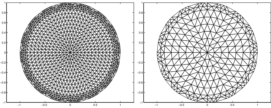
Figure 1: Element triangulation of unit circle domain. On the left is a fine finite element triangulation of the unit circle, on this triangulation sets of artificial data are generated for reconstruction later. While the coarse triangulation on the right side is the one we used for piecewise constant resistivity during reconstruction.

0 2 4 6 8 10 12

0 0.1 0.2 0.3 0.4 0.5 0.6 0.7

Iteration counts

nonlinear defect

0 2 4 6 8 10 12

0 0.1 0.2 0.3 0.4 0.5 0.6 0.7 0.8

Iteration counts

nonlinear defect

0 2 4 6 8 10 12

0 0.1 0.2 0.3 0.4 0.5 0.6 0.7 0.8 0.9 1

Iteration counts

nonlinear defect

Figure 2: The nonlinear defect error vs iterations for each parameter selection on each cases. From left to right indicates cases number. On each graphs, ’+’ is for the discrepancy principles,

(7)

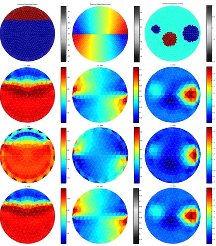
Distribusi Resistifitas Sintetis

2 Distribusi Resistifitas Sintetis

1.4

Distribusi Resistifitas Sintetis

0.5