Cluster identification and separation in the growing self-organizing map: Application in protein sequence classification.

O R I G I N A L A R T I C L E

Cluster identification and separation in the growing

self-organizing map: application in protein sequence classification

Norashikin AhmadÆDamminda Alahakoon Æ

Rowena Chau

Received: 9 January 2009 / Accepted: 19 August 2009 / Published online: 4 September 2009 ÓSpringer-Verlag London Limited 2009

Abstract Growing self-organizing map (GSOM) has been introduced as an improvement to the self-organizing map (SOM) algorithm in clustering and knowledge dis-covery. Unlike the traditional SOM, GSOM has a dynamic structure which allows nodes to grow reflecting the knowledge discovered from the input data as learning progresses. The spread factor parameter (SF) in GSOM can be utilized to control the spread of the map, thus giving an analyst a flexibility to examine the clusters at different granularities. Although GSOM has been applied in various areas and has been proven effective in knowledge discov-ery tasks, no comprehensive study has been done on the effect of the spread factor parameter value to the cluster formation and separation. Therefore, the aim of this paper is to investigate the effect of the spread factor value towards cluster separation in the GSOM. We used simple k-means algorithm as a method to identify clusters in the GSOM. By using Davies–Bouldin index, clusters formed by different values of spread factor are obtained and the resulting clusters are analyzed. In this work, we show that clusters can be more separated when the spread factor value is increased. Hierarchical clusters can then be con-structed by mapping the GSOM clusters at different spread factor values.

Keywords Cluster identificationCluster separation Unsupervised neural networksDynamic self-organizing mapProtein sequence classification

1 Introduction

The self-organizing map (SOM) [1] has been a very useful tool in discovering knowledge from data. This is due to its ability in organizing the data into groups in an unsuper-vised way and at the same time providing a two-dimen-sional visualization for the resulting groups. However, SOM’s structure is fixed and has to be determined in advance, thus its ability in finding groups in data in a more natural way is restricted. Several attempts have been made to resolve the SOM’s fixed structure problem [2, 3] including growing self-organizing map (GSOM) [4,5]. The GSOM has a dynamic structure and the spread of the map in GSOM can be controlled by using a parameter called spread factor (SF), which is an important property of the GSOM. An analyst can decide the level of spread required by manipulating the SF which accepts values from 0 to 1. The analysis could begin with a lower SF value which will give a less spread map and increasing it to get a larger spread map. By using a higher SF value, more nodes will be generated and the formation of finer clusters or subcl-usters can be observed. Study in [6] has shown that GSOM with its dynamic structure can overcome the oblique ori-entation problem caused by the fixed grid in SOM. GSOM could also reduce the map twisting and obtain maps which better represents the data distribution as compared to SOM by using its spread factor parameter.

GSOM has been used in several areas such as in text mining [7,8] and biomedical and biological data discovery [9–13]. Despite the successful implementation in the areas, so far, there has not been much study about cluster for-mation and separation in the GSOM as well as how the spread factor affects these processes. Therefore, this paper aims to investigate the effect of spread factor value to the cluster formation and separation in GSOM. This is the first N. Ahmad (&)D. AlahakoonR. Chau

formal study of the impact of spread factor parameter in GSOM. Since spread factor has been used by many researchers in several fields, we feel that a formal study providing quantitative results is timely and of high importance. We introduce the use of simple k-means algorithm and Davies–Bouldin (DB) index [14] as a method to identify the clusters from the GSOM. By using the method, the effect of the spread factor values to the cluster separation was investigated and analysed. We also present the capability of GSOM in building hierarchical clusters. In this study, two protein sequence data sets from the hemoglobin alpha chain (HBA) and cytochrome c (CYC) family have been used in the experiments.

In the following section, GSOM algorithm and its hierarchical clustering are explained in detail. Methods to carry out the quantitative analysis of the spreading-out effect in GSOM are presented in Sect.3 followed by the experimental results and discussion in Sect.4. Section5

will conclude this paper.

2 Hierarchical clustering with the growing self-organizing map (GSOM)

2.1 Growing self-organizing map (GSOM)

GSOM is a type of unsupervised neural network which based on SOM algorithm. It starts with four nodes and will continue adding nodes when it is presented with the input data. There are three phases in GSOM learning process: initialization, growing and smoothing phase. In the ini-tialization phase, weight vectors of the starting nodes are initialized with random numbers and the growth threshold (GT) is calculated. For a given data set, GT value is obtained by this equation

GT¼ DlnðSFÞ ð1Þ

whereDrefers to dimension and SF is spread factor. In the growing phase, input is presented to the network and the winner node which has the closest weight vector to the input vector is determined using Euclidean distance. The weights of the winner and its surrounding nodes (in the neighborhood) are adapted as described by

wjðkþ1Þ ¼ wherewjrefers to weight vector of nodej,kis the current

time, LR is the learning rate andNis the neighborhood of the winning neuron. During the weight adaptation, learning rate used is reduced over iterations according to the total number of current nodes. The error values of the winner

(the difference between the input vector and the weight vector) are accumulated as follows:

Total Error; TEi¼

dimension, xi,jandwi,jare the jth dimension of input and

weight vectors of the node i, respectively. The new nodes will only grow from a boundary node. This will happen when the total error exceeds the growth threshold. The weights for the new nodes are then initialized to match the neighboring node weights. For non-boundary nodes, errors are distributed to the neighbors. The growing phase is repeated until all input has been presented and can be terminated once the node growth has reduced to a mini-mum value.

In the smoothing phase, no node will be grown and only weight adaptation process is carried out. The learning rate is reduced and weight adaptation is done in a smaller neighborhood compared to the growing phase.

In GSOM, when a higher spread factor value is used the map will expand and more branching-out of the map can be observed. This provides the user with an easy way to identify the groups or clusters from the map. Even though clusters can be manually identified from the map visuali-zation, an automated method to identify the clusters would be an advantage. It has been suggested in [4] that auto-mated cluster identification is needed in some situations, such as when the cluster boundary is not clear. Data skel-eton modeling (DSM) [4, 15] has been proposed as an automated method to identify clusters in GSOM. The model is built by tracing along the path of the node gen-eration in GSOM. The separation of the clusters can be made by removing the path segment that has the largest distance value from the data skeleton. If more clusters are needed, the removal process can be continued. Dynamic SOM Tree [16] is another method used for identifying clusters from GSOM. In this method, at least two maps with different resolutions (different values of spread fac-tor), must first be obtained. By mapping the nodes that contain the same input data between maps at consecutive layers, clusters as well as their merging and separation can be visualized.

not be in proportion to the distribution of the clusters. Figure1a shows an optimal map when the grid size is proportional to the data distribution, and a distorted map (Fig.1b) when the grid tries to fit into the data distribution. In Fig.2, the SOM and GSOM grid after presented with the star data are shown.

As can be seen from Fig.2, it is apparent that GSOM represents the data distribution more accurately than SOM. It can be seen that even at low spread factor value (for example, 0.1), nodes have followed the distribution of the data and a clear star-shaped grid has been obtained. The map becomes more dense with higher spread factor values as more nodes have been grown. It can be observed that with the node addition, a map grid that better conforms with the data distribution has been generated. In contrast to GSOM, even when the size of the SOM grid is increased, the nodes could not represent the overall data distribution. It has been noted in [6] that in order to get a map size that in proportion to the data distribution, the map size could be initialized according to the data values or dimension; however, this will require the data analyst to have knowl-edge about the data before hand which is not practical in many situations.

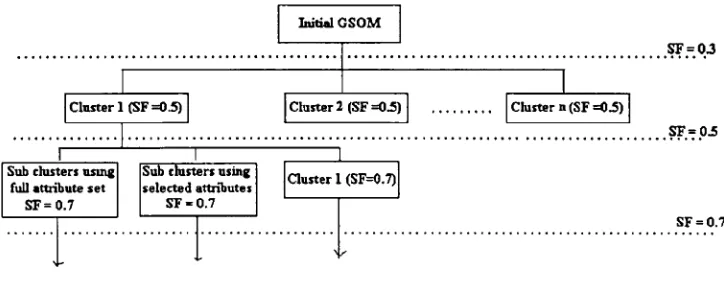
2.3 Hierarchical clustering using the spread factor Spread factor value can be used to control the spread of the map. By using a higher SF, map is expanded and more detailed clusters or the formation of subclusters can be obtained. As GSOM can generate clusters at different granularities by utilizing the SF, hierarchical clustering on a data set can be carried out. Figure3 illustrates the hier-archical clustering with GSOM.

In Fig.3, hierarchical clustering is done through expanding Cluster 1 at SF 0.5. By using a SF value of 0.7, three subclusters have been obtained. The clustering process can be repeated for all clusters or any cluster of interest at a higher SF value if the data analyst needs to get an extended analysis of the cluster. The example of hier-archical clustering using GSOM from previous studies can be found in [5] (animal data set) and [11] (sleep apnea data set).

3 Quantitative analysis of the spreading-out effect and hierarchical clustering usingk-means algorithm

The use of automated cluster identification in cluster anal-ysis process has several advantages. Clusters in GSOM can be identified by observing the map output in which nodes associated with a particular group are separated from other groups by dummy nodes (non-hit nodes). However, deter-mining the clusters visually can be difficult especially in a low spread map as the map contains lesser number of nodes including the dummy nodes. In this case, two distinct clusters may not be separated by the dummy nodes and some of their nodes are located next to each other resulting in an unclear boundary. The use of an automated cluster identification method is beneficial as it could reduce the ambiguity in determining the cluster boundary which could Fig. 1 The spread-out effect in SOM.aOptimal grid,bgrid does not

conform to data distribution (distorted map/oblique orientation) [6]

not be identified by visual inspection. The automated method also means that human involvement can be reduced in the cluster analysis, thus, making the process faster. In addition, it will facilitate the online learning and data monitoring system where they require cluster analysis to be carried out continuously in online manner. In this section, we describe the use ofk-means algorithm as an automated method to identify the clusters and to investigate the spread-out effect in GSOM. After that the building of hierarchical structure from the identified clusters is explained.

3.1 Cluster identification

Simplek-means clustering has been used in this study as a method to identify the clusters and investigate the spread-out effect in the GSOM.k-means is a partitional clustering algorithm that uses minimum squared error criterion in grouping the data [17]. The algorithm is as follows: a. Determine the number of clusters,k

b. Initialize the centroids (cluster centers) values withk randomly chosen input samples

c. Find the closest cluster (smallest distance to centroid) for each sample and assign the sample to that cluster d. Update the centroid for each cluster with new values e. Repeat until convergence, or if there is minimal or no

change in the cluster membership.

In this process, the weight values for each hit node (node which has at least one input data mapped to it) obtained from the GSOM clustering were used as samples for the k-means clustering.k-means clustering was carried out for all GSOM output with number of clustersk, from two to ten. Ask-means clustering is sensitive to the centroid ini-tialization, for eachkwe run the algorithm for ten iterations with different centroid values that were randomly chosen from the input samples. The best cluster partitioning for eachkwas selected by using a cluster validity index called the DB index [14] which measures the within-cluster var-iation and between-cluster varvar-iation for the resulting clus-ters. By using the index, the best partitioning minimizes the following function:

DB¼1_n X

n

i_¼1;i6¼j

max SiþSj d ci;cj

!

ð4Þ

where n is the number of clusters, Si and Sj are within

cluster variations (average distance of samples in each cluster to the cluster center) in clusteriandj, respectively, and d(ci, cj) is the between-cluster variation (distance

between cluster centeriandj).

For every spread factor value, the k-means clustering process has been carried out five times. Then, the lowest DB index values and their corresponding number of clus-ters across experiments (five runs ofk-means) were taken for each specified spread factor. The range for the number of cluster in which the lowest DB index value was taken is based on the number of samples,NwhereNis the number of hit nodes in GSOM at a particular spread factor. The range used is from k=2 to ffiffiffiffiN

p

as suggested by Vesanto et al. in [18].

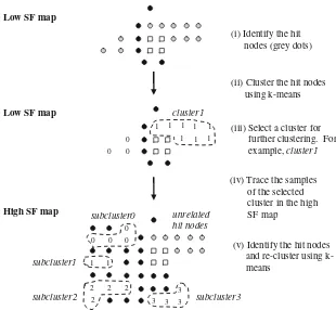
3.2 Spreading-out effect and hierarchical clustering The effect of the spread factor parameter to the separation of clusters in GSOM as well as the GSOM capability in building hierarchical clusters were investigated by observing the clusters by using the k-means algorithm. To construct hierarchical clusters, a similar method as described in [5] has been used. However, instead of iden-tifying the clusters visuallyk-means algorithm was applied to discover the clusters and subclusters formation. The following figure shows the method to build hierarchical clusters for GSOM using thek-means algorithm.

Steps for building the hierarchical clusters as shown in Fig.4can be summarized as follows:

(i) Identify the hit nodes from a low SF map (grey dots) (ii) Runk-means fork₌2 tok₌pffiffiffiffiNusing hit nodes as samples. Choose the best partition (k) by selecting the lowest DB index.

(iii) Select a cluster for further clustering.

(iv) Trace the samples of the selected cluster in the higher SF map.

(v) Runk-means for k₌2 tok₌pffiffiffiffiN: Samples are hit

nodes in higher SF map which contain samples from the selected cluster in low SF map. Choose the best partition (k) by selecting the lowest DB index.

4 Experimental results

4.1 Data preparation

In the experiments, we have used two data sets of protein sequences; hemoglobin alpha chain (HBA) and cytochrome c (CYC). These data sets were downloaded from the SWISS-PROT database release 13.1 [19]. HBA and CYC sequences have been used in protein classification using SOM [20] and phylogenetic analysis using self-organizing tree network (SOTA) [21]. Phylogenetic analysis is a method to infer relationship between species or organisms. According to evolutionary theory, HBA and CYC families evolve slowly compared to other families, thus the patterns are more conserved. Clustering of the sequences from these families will result in the sequences being grouped according to their species or taxonomic groups, which is useful in phylogenetic analysis where evolutionary rela-tionship among the species or organisms can be inferred.

In [20], different SOM sizes have been used in clustering protein sequences. The effect of using different learning parameter values and protein sequence representations to the map also has been investigated. The construction of

phylogenetic tree of protein families using SOTA algorithm was the main objective in [21]. Unlike SOM, SOTA can generate nodes dynamically and give a tree structure as the final clustering output. Results from the experiments showed that this algorithm is capable of building the phy-logenetic trees for several protein families such as CYC, HBA, triosephosphate isomerase and also a mixture of interleukins and receptors.

The detail information about each data set is shown in Table1.

In this study, we used both data sets to analyze the cluster formation and separation in GSOM as well as dif-ferent level of clustering that can be achieved when using various spread factor values. After the clustering process completed, only main groups and subgroups were com-pared with the expected groups as shown in Table1. As the

0

(iii) Select a cluster for further clustering. For example, cluster1

(i) Identify the hit nodes (grey dots)

(ii) Cluster the hit nodes using k-means

(v) Identify the hit nodes and re-cluster using k-means

(iv) Trace the samples of the selected cluster in the high SF map

Fig. 4 Building hierarchical clusters for GSOM using the k-means algorithm

Table 1 The description of the data sets used in the study

Data set Number of sequences

209 5 Mammals (135), birds (39),

fishes (23), reptiles (9), amphibians (3)

Cytochrome c(CYC)

120 9 Plants (30), fungi (21),

objective of the study is not the reconstruction of phylo-genetic tree as in [20], we do not have a complete phylo-genetic tree as the final outcome of the analysis.

4.2 Feature extraction and encoding of the protein sequences

Feature extraction and encoding of protein sequences must be done before the clustering process begins. Each protein sequence contains the combination of 20 basic amino acids abbreviated as A, C, D, E, F, G, H, I, K, L, M, N, P, Q, R, S, T, V and W. Each amino acid has its own physico-chemical properties that can influence the structure and function of a protein. Apart from taking each individual amino acid as feature, amino acid physicochemical prop-erties such as exchange group, charge and polarity, hydrophobicity, mass, surface exposure and secondary structure propensity also can be used in order to maximize the information extraction from the protein sequences [22,23].

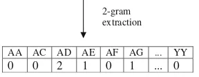
For the encoding of the protein sequences, two approaches called direct and indirect encoding method have been used. Direct encoding method employs binary representation (0 and 1) to represent each amino acid [24]. For example, to represent an amino acid, a single one is put into a specific vector position and other 19 positions will be set to zero. This technique requires pre-alignment of the sequences to make the input length equal. During the alignment process, gaps may be inserted in the sequence. To represent the gap, all positions can be set to zero or vector size of 21 can be used with one position is reserved for the gap. The advantage of using the direct encoding method is it could preserve the position information, however, it results in a sparse and large size (dimension) input vector. The indirect method involves the encoding of global information from the protein sequence by using residue frequency or n-gram method. In the n-gram method, the frequency of amino acid occurrence for n consecutive residues is calculated along the sequence like a sliding window. Amino acid dipeptide composition or 2-gram method has been used in [20,21, 25]. In [21,26,

27], variousn-grams with different sizes and features have been applied in the protein sequence encoding. Apart from n-grams that are generated from individual amino acids, the authors also have replaced each of the amino acid letters according to physicochemical properties and then generated n-grams from the sequence. In the experiment, they also have combined different types and sizes of n-grams into one set of input vectors. The indirect method does not require alignment of the sequences and can be used to extract short motifs that may be significant to the protein function. However, the order of sequence is not taken into consideration which means the position

information will be lost. To overcome the limitation, in [27], an additional vector that represents the position of the n-gram pattern has been included in the sequence encoding. Results showed that the addition of the position vector has improved the performance of the encoding method.

In this study we have employed the 2-gram extraction method to encode the amino acids. This 2-gram patterns extraction has resulted in 202 or 400 input dimensions. Example of the 2-gram extraction for a protein sequence is shown in Fig. 5.

After the 2-grams extraction method completed for every protein sequence in the data sets, the frequency values were scaled to between 0 and 1 before presenting them to the GSOM. The effect of using different encoding methods is beyond the scope of this paper, therefore, 2-gram encoding method is simply chosen as it has been employed as one of the encoding methods to cluster the protein sequences using self-organizing map in the previ-ous studies.

4.3 GSOM clustering

GSOM clustering requires the settings of several parame-ters such as spread factor, learning rate, factor of distri-bution (FD) andRvalue. We have used learning rate of 0.1, FD of 0.3 and Rof 0.4 for all experiments. For each data set, we run the experiments each with various number of spread factors values (small to large). In the smoothing phase, a smaller learning rate value (0.05) has been used. Pre-investigation showed that for all datasets, the node growth has stabilized and learning convergence can be achieved before reaching 50 iterations. Therefore, we have fixed the number of iterations in GSOM learning to be 50 throughout the experiments.

4.4 Cluster visualization using GSOM

The visualization of the output obtained for HBA sequen-ces at spread factor 0.1 and 0.95 are shown in Figs.6and7, respectively. From the figures, white square nodes repre-sent the four initial nodes and nodes labeled with numbers

Protein sequence>P18970|HBA_AILME Hemoglobin subunit alpha - Ailuropoda melanoleuca (Giant panda).

MVLSPADKTNVKATWDKIGGHAGEYGGEALERTFASFPTTKTYFPHFDL

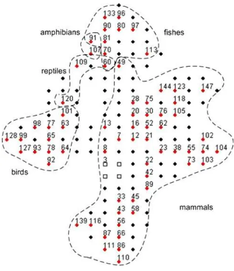
indicate the hit or winner nodes. Based on the visualization from both figures, we can see that GSOM has successfully identified the patterns in the sequences and clustered them into their expected groups. Almost all sequences from the same animal group have been positioned in nodes that are adjacent to each other, confirming the capability of GSOM in preserving the topology of the map. Figure6also shows that mammals have been well separated from the other animal groups and all nodes consist of only mammal sequences. However, for other animal groups, some nodes were found to have sequences from other animal groups, for example node 26 (two birds and three reptiles), 12 (two fishes, two amphibians and two reptiles) and 15 (21 fishes and one amphibian). As illustrated in Fig.7, at SF 0.95, more nodes have been generated and a clearer separation of the animal groups can be observed. It is also interesting to see that only two nodes (node 60 and 91) contain sequences from more than one animal group. We can also observe the change in the shape of the map where the groups have been spread out further into certain directions.

Observation on the clustering of the sequences into each node for the visually identified animal groups also has been done. Results showed that GSOM also could classify the animals into their specific groups or subgroups. More spe-cific type of animals also has been located into separate nodes. Figure8 presents an example of some subgroup formations as identified from the mammal group. From the figure, we can see that primates have been clustered into nodes that are positioned next to each other in a specific region. The primate group consists of loris, colobus, chim-panzee, orangutan, gorilla, human, sphinx, lemur, macaques, monkeys, sapajou, tamarin and capuchin and other primates. Figures9 and 10 present GSOM for CYC data set at spread factor 0.1 and 0.95, respectively. As can be seen from the figures, at SF 0.1 there is a clear separation for plants and

fungi groups and nodes contain only sequences that belong to their groups. However, bird, mammal, amphibian and reptile sequences were found to be clustered together in node 2, 3 and 4. Most of the fish and insect sequences are clustered into node 12 and 6 but they are mixed with sequences from ‘‘others’’ group. As shown in Fig. 10, at spread factor 0.95, more nodes have been grown for each group. Similar to spread factor 0.1, fungi and plant groups are well separated from other groups. It is also interesting to see that insect and fish groups overlap with ‘‘others’’ group in SF 0.95, similar to SF 0.1. This indicates the closeness of the fish and insect sequence patterns to each other. Bird, mammal, amphibian and reptile groups also show the same behaviour. Even though bird sequences are all clustered into the same node Fig. 6 GSOM clustering for HBA data set at spread factor 0.1

Fig. 7 GSOM clustering for HBA data set at spread factor 0.95

(node 86), they are still located in a same region with mammal, reptile and amphibian sequences.

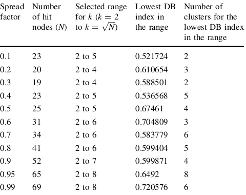
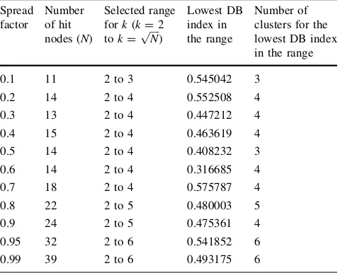
4.5 Investigation on the effect of spread factor to the cluster formation and separation in GSOM The results obtained from the experiments for HBA data sets are shown in Table2and Fig.11while for CYC data set in Table3 and Fig.12. We have used DB index to determine the best partitioning and appropriate number of

cluster for the GSOM in each spread factor. The DB index value shown in the results is the lowest DB index values from five runs ofk-means experiments (kbetween two and

ffiffiffiffi

N p

) in each spread factor. From Tables2 and 3, we can see that small number of hit nodes has been obtained in lower spread factors and continue to increase when the spread factor value increases. This effect is caused by growth threshold (GT) value of GSOM (1). The use of a low spread factor will result in a high GT causing a lesser growth of nodes and a high spread factor yields a low GT, allowing more nodes to grow and thus, expanding the size of the map. This can be seen in the clustering output of the HBA data set from Figs.6 and 7. As the number of hit nodes differs in each spread factor, different range has been used in each spread factor depending on the total number of hit nodes. On overall, for both data sets, values for the number of clusters were shown to have increased when the spread factor used was higher. Figures 11and12illustrate Fig. 9 GSOM clustering for CYC data set at spread factor 0.1

Fig. 10 GSOM clustering for CYC data set at spread factor 0.95

Table 2 Number of clusters based on spread factor and DB index values for HBA data set (kis number of clusters)

Spread factor

Number of hit nodes (N)

Selected range fork(k=2 tok=pffiffiffiffiN)

Lowest DB index in the range

Number of clusters for the lowest DB index in the range

0.1 23 2 to 5 0.521724 2

0.2 20 2 to 4 0.610654 3

0.3 19 2 to 4 0.588501 2

0.4 23 2 to 5 0.536568 5

0.5 25 2 to 5 0.67461 4

0.6 31 2 to 6 0.704809 3

0.7 34 2 to 6 0.583779 6

0.8 41 2 to 6 0.599404 5

0.9 52 2 to 7 0.599871 4

0.95 65 2 to 8 0.6492 8

0.99 69 2 to 8 0.720576 6

0 1 2 3 4 5 6 7 8 9

0 0.1 0.2 0.3 0.4 0.5 0.6 0.7 0.8 0.9 1

Spread Factor (SF)

No. of Clusters

this trend. This finding confirms the effect of spread factor values to the separation or splitting of clusters as shown by the manual observation in Sect.4.4, where subgroupings of node or subclusters were found when a higher spread factor value was used.

The spread factor values used in the experiment are arbitrarily chosen—from low to high (range of SF value is between 0 and 1). The purpose of the SF is to generate different number of clusters, where such clustering may appear. In this analysis, we also have presented a method for identifying a potentially ‘best’ number of clusters. As such the SF or SFs, which generate this optimal clustering, will be the ‘best SF’ for the application.

4.6 Cluster separation and hierarchical clustering

To demonstrate the proposed method, we used HBA data set and its GSOM output at SF 0.1 and SF 0.95. The

visualization of the clustering output in spread factor 0.1 for HBA data set is shown in Fig.6. By taking the hit node weight values as samples for the k-means algorithm as described in Sect.3.1, the lowest DB index acquired for SF 0.1 is 0.521724 and its corresponding number of cluster is two (cluster range,k₌2 tok₌5). Figure13a shows that the map has been partitioned into two sections with group 0 on the right and group 1 on the left side of the map. Comparing Figs. 6 and 13a, it can be seen that group 0 consists of all mammals, all fish, all amphibians and some reptile sequences whereas group 1 contains bird and other reptile sequences. To examine the separation of the clusters in higher spread factor value, the sequences which occu-pied the nodes in group 0 were traced in the SF 0.95 map. By clustering the hit nodes in SF 0.95 map which contain sequences from group 0 usingk-means method, clusters as shown in Fig.13b have been obtained. We have run the k-means algorithm five times and selected the lowest DB index value for cluster number range from two to seven. Table 3 Number of clusters based on spread factor and DB index

values for CYC data set (kis number of cluster)

Spread

Fig. 12 Spread factor and number of clusters for CYC data set shown by linear regression graph

The best number of partitions is seven which has the DB index value of 0.627262.

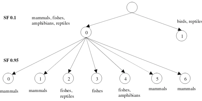
Based from the output obtained using the k-means algorithm, the hierarchical clusters for HBA sequences can be visualized as in Fig.14. It is observed that by using a high spread factor value, the separation of clusters in GSOM can be achieved. The breakdown of the sequences in each cluster at SF 0.95 is shown in Table4. We show only the animal names to represent the sequences to ease the understanding.

From the distribution of sequences shown in Table4, we can see that the main groups of animals have been suc-cessfully identified. It is interesting to see, in case of mammal sequences as they have been divided into four clusters (0, 1, 5 and 6). Based on general observation, these clusters may be labelled as: primate group (cluster 0), meat-eating mammals (cluster 5) and non meat-eating mammals (cluster 6). As for cluster 1, it contains only opossum sequences. On the map this cluster is located near the fish and reptile clusters and is separated from other mammal clusters. This finding suggests that the opossum sequence pattern may have high similarities with the fish and reptile sequence pattern. A closer look to each node of the clusters reveals that most of the animals which are similar have been placed in the same node. For example in cluster 5, black bear, polar bear, sun bear, seal, red panda and giant panda are grouped into the same node.

5 Conclusion

This paper has investigated the effect of spread factor value on the separation of cluster in GSOM. We have shown that by using a basic k-means algorithm and the DB validity index, clusters in GSOM can be identified. In previous studies which employed self-organizing map to classify protein sequences [20, 25], clusters were identified by visual inspection. However, determining the clusters from the map can be a difficult task if the winning nodes are near

to each other. Furthermore, the formation of clusters can only be confirmed if we already have knowledge about the groups that can be obtained from the data. The use of

1 0

0 1 2 3 4 5 6

mammals, fishes,

amphibians, reptiles birds, reptiles

SF 0.1

SF 0.95

mammals mammals fishes, fishes mammals mammals

reptiles

fishes, amphibians

Fig. 14 Hierarchical clusters obtained from GSOM SF 0.1 and SF 0.95 for HBA data set (only group 0 is used in the process)

Table 4 Distribution of HBA sequences in each cluster at SF 0.95

Cluster Animala

0 (sapajou, moustached tamarin, brown-headed tamarin, cotton-top tamarin, marmoset, spider monkey, capuchin), (slender loris, slow loris), red colobus, (chimpanzee, orangutan, pygmy chimpanzee, gorilla, human), (rhesus macaque, Japanese macaque, green monkey), (sphinx, lemur, stump-tail macaque), (crab eating macaque, toque macaque, olive baboon, assam monkey, langur, mangabey, gelada baboon, yellow baboon, pig-tailed macaque)

1 North American opossum, short-tailed gray opossum

2 (dogfish, sea snake, Texas indigo snake, viper)

3 (carp, desert sucker, spot, goldfish, eel), (Artedidraco orianae, Pogonophryne scotti), salmon, (zebrafish, red gurnard), (bald rockcod, Antarctic dragonfish, emerald rockcod, flathead, dragonfish, tuna), (shark, spotless smooth hound)

4 (newt, latimeria, axolotl), lungfish, frog, (eaton’s skate, stingray)

5 Sloth, mole, (black bear, polar bear, sun bear, seal, red panda, giant panda), hedgehog, (aardwolf, hyena), (badger, coati), (polecat, otter, ferret, walrus, seal, raccoon, mink, ratel, otter), civet, (dog, wolf, red fox, coyote), (amur leopard, northern Persian leopard, Sumatran tiger, jaguar, lion, cat)

6 (African elephant, Indian elephant), (donkey, Przewalski’s horse, mountain zebra, horse, kulan), deer, vicugna, whale, hyrax, (Bactrian camel, guanaco, Arabian camel, alpaca, rabbit, llama), pig, hippopotamus, (sheep, elk, gayal, bison, goat, barbary sheep, chiru, reindeer), (dolphin, whale), (muskrat, hamster, rat), shrew, (armadillo, kudu), (platypus, hedgehog, manatee), gambia rat, mouse, guinea pig, (suslik, Arctic ground squirrel, marmot, Townsend’s squirrel), (wallaby, kangaroo, quoll), white rhinoceros, (pallid bat, tomb bat, Egyptian fruit bat, California big-eared bat, Indian short-nosed fruit bat, black flying fox, cave bat, Australian ghost bat, grey-headed flying fox), (chocolate-wattled bat, Japanese house bat, tarsier), molerat, (gundi, shrew)

automatic identification method could expedite as well as increase the accuracy of the cluster analysis process and enable unknown or possible clusters to be found.k-means algorithm and the DB validity index provide an automated way in discovering clusters from the GSOM as demon-strated in this study. By using the proposed method, we have quantitatively confirmed that separation of cluster happens when a high spread factor value is used.

In this paper, the capability of GSOM in building hier-archical clusters also has been demonstrated. This study indicates the potential of GSOM in performing bioinfor-matics tasks, which require hierarchical representation such as in phylogenetic analysis and protein family classifica-tion. In this method we have usedk-means algorithm as it is easy to implement and has been used widely as a clus-tering tool. However, there are some issues pertaining to its performance such as its sensitivity to the initial centroids, convergence to global optimum and sensitivity to outliers and noise as reported in [28]. It is suggested that in future, more analysis to be done in order to evaluate its effec-tiveness in finding clusters in the GSOM by using the proposed method.

There are also other encoding techniques and different features of amino acid that can be used as input to the clustering process, however, in this study we simply used 2-gram encoding method which is the frequency of occu-rence of two consecutive amino acids from a protein sequence. The main objective of this paper is the demon-stration and analysis of the spread factor parameter which is unique to the GSOM algorithm, therefore, we do not take into consideration the effect of different encoding methods to the cluster formation and separation. In addition, the 2-gram encoding technique has been used successfully in other published papers [20,21,25] related to the clustering of protein sequences. We hope to include other feature extraction and encoding methods of protein sequences in future work. As we are focusing more on the investigation of the effect of spread factor value to the cluster formation in GSOM rather than the quality of the clustering process, evaluation of the algorithm in terms of precision or com-putation time as well as comparison of the results with other related papers were not included in the analysis.

References

1. Kohonen T (1990) The self-organizing map. Proc IEEE 78:1464– 1480

2. Fritzke B (1994) Growing cell structures: a self-organizing net-work for unsupervised and supervised learning. Neural Netw 7:1441–1460

3. Blackmore J, Miikkulainen R (1993) Incremental grid growing: encoding high-dimensional structure into a two-dimensional

feature map. In: IEEE international conference on neural net-works, pp 450–455

4. Alahakoon LD (2000) Data mining with structure adapting neural networks. In: School of computer science and software engi-neering. Monash University, pp xvii, 286 leaves

5. Alahakoon D, Halgamuge SK, Srinivasan B (2000) Dynamic self-organizing maps with controlled growth for knowledge dis-covery. IEEE Trans Neural Netw 11:601–614

6. Alahakoon LD (2004) Controlling the spread of dynamic self-organising maps. Neural Comput Appl 13:168–174

7. Amarasiri R, Alahakoon D,Smith KA (2004) HDGSOM: a modified growing self-organizing map for high dimensional data clustering. In: Fourth international conference on hybrid intelli-gent systems, 2004 (HIS ‘04), pp 216–221

8. Zheng X, Liu W, He P, Dai W (2004) Document clustering algorithm based on tree-structured growing self-organizing fea-ture map advances in neural networks—ISNN 2004, pp 840–845 9. Hsu AL, Tang S-L, Halgamuge SK (2003) An unsupervised hierarchical dynamic self-organizing approach to cancer class discovery and marker gene identification in microarray data. Bioinformatics 19:2131–2140

10. Chan C-KK, Hsu AL, Tang S-L, Halgamuge SK (2008) Using growing self-organising maps to improve the binning process in environmental whole-genome shotgun sequencing. J Biomed Biotechnol 2008:10

11. Wang H, Azuaje F, Black N (2004) An integrative and interactive framework for improving biomedical pattern discovery and visualization. IEEE Trans Inf Technol Biomed 8:16–27 12. Zheng H, Wang H, Azuaje F (2008) Improving pattern discovery

and visualization of SAGE data through poisson-based self-adaptive neural networks. IEEE Trans Inf Technol Biomed 12:459–469

13. Wang H, Zheng H, Hu J (2008) Poisson approach to clustering analysis of regulatory sequences. Int J Comput Biol Drug Design 1:141–157

14. Davies DL, Bouldin DW (1979) A cluster separation measure. IEEE Trans Pattern Anal Mach Intell 1:224–227

15. Amarasiri R, Wickramasinge K,Alahakoon D (2003) Enhanced cluster visualization using the data skeleton model. In: 3rd international conference on intelligent systems design and application (ISDA), Oklahoma, USA

16. Hsu A, Alahakoon D, Halgamuge SK, Srinivasan B (2000) Automatic clustering and rule extraction using a dynamic SOM tree. In: Proceedings of the 6th international conference on automation, robotics, control and vision, Singapore

17. Jain AK, Murty MN, Flynn PJ (1999) Data clustering: a review. ACM Comput Surv 31:264–323

18. Vesanto J, Alhoniemi E (2000) Clustering of the self-organizing map. IEEE Trans Neural Netw 11:586–600

19. Boeckmann B, Bairoch A, Apweiler R, Blatter M-C, Estreicher A, Gasteiger E, Martin MJ, Michoud K, O’Donovan C, Phan I, Pilbout S, Schneider M (2003) The SWISS-PROT protein knowledgebase and its supplement TrEMBL in 2003. Nucl Acids Res 31:365–370

20. Ferran EA, Pflugfelder B, Ferrara P (1994) Self-organized neural maps of human protein sequences. Protein Sci 3:507–521 21. Wang H-C, Dopazo J, De La Fraga LG, Zhu Y-P, Carazo JM

(1998) Self-organizing tree-growing network for the classifica-tion of protein sequences. Protein Sci 7:2613–2622

22. Wu CH, McLarty JW (2000) Neural networks and genome informatics. Elsevier, Oxford, Amsterdam

24. Andrade MA, Casari G, Sander C, Valencia A (1997) Classification of protein families and detection of the determinant residues with an improved self-organizing map. Biol Cybern 76:441–450 25. Ferran EA, Ferrara P (1991) Topological maps of protein

sequences. Biol Cybern 65:451–458

26. Wu CH, Ermongkonchai A, Chang T-C (1991) Protein classifi-cation using a neural network database system. In: Proceedings of

the conference on analysis of neural network applications. ACM, Fairfax, Virginia, United States

27. Wu C, Whitson G, McLarty J, Ermongkonchai A, Chang TC (1992) Protein classification artificial neural system. Protein Sci 1:667–677