Generating concept trees from dynamic self-organizing map.

Generating Concept Trees from Dynamic

Self-organizing Map

Norashikin Ahmad, Damminda Alahakoon

Abstract—Self-organizing map (SOM) provides both clustering and visualization capabilities in mining data. Dynamic self-organizing maps such as Growing Self-organizing Map (GSOM) has been developed to overcome the problem of fixed structure in SOM to enable better representation of the discovered patterns. However, in mining large datasets or historical data the hierarchical structure of the data is also useful to view the cluster formation at different levels of abstraction. In this paper, we present a technique to generate concept trees from the GSOM. The formation of tree from different spread factor values of GSOM is also investigated and the quality of the trees analyzed. The results show that concept trees can be generated from GSOM, thus, eliminating the need for re-clustering of the data from scratch to obtain a hierarchical view of the data under study.

Keywords—dynamic self-organizing map, concept formation, clus-tering.

I. INTRODUCTION

S

elf-organizing map (SOM) [1] is an unsupervised learning method based on artificial neural networks. It can produce a two-dimensional map from a high dimensional data and has a topology-preserving property that makes cluster analysis be made easier. SOM is very useful tool in data mining however; it suffers from several limitations mainly because of its fixed structure whereby the number of nodes has to be determined in advance.

The Growing Self-organizing Map (GSOM) algorithm [2] has been developed to enhance the ability of SOM in repre-senting the input patterns. The learning of GSOM is similar to SOM but the structure is dynamic enabling clusters to be formed without restriction on the map size. GSOM has been successfully applied in several applications such as in text mining [3], bioinformatics data mining [4], [5] and also in intelligent agent framework [6].

Hierarchy is one of the structures that are commonly used to discover knowledge from data. It is a convenient way to visualize the multiple-level relationship between the data as well as to summarize the data from general to specific order. Traditional agglomerative or divisive hierarchical algorithms have some disadvantages when used with large datasets. Not only do they require multiple iterations but the output is also difficult to interpret. It may result in a huge tree whereby the nodes and levels cannot be visualized effectively. In the traditional hierarchical clustering, each instance is in its own cluster at the lowest level of the hierarchy. Therefore, to examine all of the clusters for a large dataset in the hierarchy would be a difficult task. This problem has been highlighted by Chen et al [7] by clustering a large protein sequence

Norashikin Ahmad and Damminda Alahakoon are with the Clayton School of IT, Monash University, Australia, e-mail: norashikin.ahmad, dam-minda.alahakoon@infotech.monash.edu.au

database. They have proposed an approach to summarize the hierarchy by flattening the homogeneous clusters according to some statistical criteria, resulting in fewer non-leaf nodes and has more matches against the target clusters, protein families defined in the InterPro.

Another type of hierarchical structure used in knowledge discovery is concept hierarchy. Concept hierarchy according to Han and Kamber [8] is a structure that can be used to represent domain knowledge such that attributes and attribute values are organized into different level of abstractions. Concept hierarchy is also used in Michalski’s conceptual clustering model following the concept of knowledge organization in human learning [9]. In the model, knowledge is represented in a concept hierarchy where instances are classified in top-down fashion where top signifies more general concepts and is more specific towards the bottom of the hierarchy. Al-though conceptual clustering organizes knowledge in a form of hierarchy similar to other hierarchical clustering techniques, the structure is different as each node in the hierarchy has a conceptual description allowing easier interpretation of the cluster. This is the most important feature of conceptual clustering that distinguishes the method from the others. The use of conceptual description in classification model is also useful in order to discover profiles and to better understand how the system arrives at a particular solution.

Acknowledging the importance of hierarchy in knowledge discovery, in this paper, a method to generate concept trees from GSOM is proposed and investigated. The building of the concept tree from GSOM has several advantages. Firstly, a hierarchical structure can be obtained from GSOM without having to re-run the hierarchical algorithm on the data set. Secondly, the hierarchy is also summarized (as GSOM clus-ters), thus, the visualization and cluster interpretation process is made easier since SOM-based clusters are an accepted data visualization technique. Thirdly, by constructing the hierarchy from the GSOM we get both advantages of cluster visualiza-tion based on self-organizing map and also the hierarchical clusters. This will help analyst to better understand about the structure of the data as well as the relationship between the clusters.

In the next section, we present the detail of GSOM algo-rithm followed by the building of the concept tree process in Section 3. In Section 4, experimental results are described. Section 5 will conclude this paper.

II. GROWINGSELF-ORGANIZINGMAP

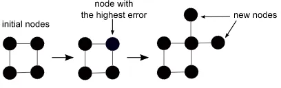
Fig. 1. The process of growing nodes in GSOM

is presented with input. Figure 1 shows the growing of nodes in GSOM. The topology of GSOM could be rectangular or hexagonal [5]. GSOM has a parameter called spread factor (SF) which can be used to control the spread of the map. The SF value (ranged from 0 to 1) is determined by the analyst before the training begins. A low SF value will give a less spread map whereas a high SF value gives a more spread map. If the analyst wants to observe a finer cluster or subclusters, a higher SF value can be used.

The growing of nodes in GSOM is actually attributed to the growth threshold (GT), which utilizes the SF value. The GT value is calculated as follows.

GT =−D×ln(SF) (1)

whereD is the dimension.

There are three learning phases in GSOM process; initializa-tion, growing and smoothing phase. In the initialization phase, weight vectors of the initial nodes are initialized with random values (0 to 1). The growing phase starts with presenting an input vector to the network. The weight adaptation at iteration tis described as follows.

∆wij(t) =

α(t)LR(t) (xi(t)−wij(t)), j ∈Nt 0, j /∈Nt (2)

whereα(t)andLR(t)are the learning rate and the neighbor-hood function at iteration t, respectively. In GSOM algorithm, the learning rate decay is based on the total number of nodes at iteration t. The learning rate is reduced as shown in the following equation.

LR(t+ 1) =α×ψ(n)×LR(t) (3)

where α is the learning rate decay, LR(t) is the learning rate at iteration t and ψ(n) is a function that takes n, the current number of nodes. The error values of the winner that is the difference between the input vector and the weight vector will be accumulated over iterations. An example of error accumulation for nodeiis described as follows.

T Ei=

whereHi is the number of hits, D is the dimension of the data,xi,j andwi,j are thejth dimension of input and weight vectors of nodeirespectively. The total error value is used to indicate the node growth in GSOM.

The smoothing phase in GSOM is the fine tuning of the quantization error in the network whereby no nodes will be grown and only weight adaptation process is carried out.

III. BUILDING THECONCEPTTREE

GSOM algorithm is used as the starting point to cluster all the instances in the initial dataset. Once the map has been generated, clusters from GSOM are identified by using the cluster identification method as in [4]. The identification method is carried out by clustering the hit nodes on the map with the k-means algorithm. The k-means algorithm will be run from k=2 to k= √N, where N is the total number of hit nodes from the map. The best k is selected by using the Davies-Bouldin (DB) index. The identified clusters from GSOM become the children of the root, creating the first level of the tree. The statistics of each cluster in the level are calculated and stored, becoming the feature or concept for that cluster. The statistics are obtained from the hit nodes in the cluster including number of hit nodes mapped to the cluster as well as the average, sum and sum of square of value for each dimension. These clusters are refined further to get the subsequent levels of the tree. To get the second level, the following algorithm is performed for each cluster (c1i) in the first level.

A. Refining Clusters at Level 1

In this step, following the minimum spanning tree algorithm (MST) each hit node in the cluster are linked to the node that is closest, using the Euclidean distance. We may find groups of nodes that are linked together forming a set of new clusters. These clusters will be used to form level two of the initial concept tree. However, if there is only one hit node in the cluster passed from level one, the previous step will not be performed, instead, the hit node itself will directly becomes the child of cluster c1i in the tree. If the cluster c1i does not break up into clusters at level 2 (all hit nodes in cluster c1ilink to each other), we make all the hit nodes as children to clusterc1i. This means the hit nodes have formed a tight cluster which does not need to be refined further in the next step. We do not create the new cluster,c2i in level 2 forc1i to avoid one to one cluster mapping between clusterc1i and c2i. The algorithm to refine the first level of the tree is shown in Algorithm 1.

B. Refining Clusters at Level 2

Input: clusterc1i

Output: sub clusters forc2i at Level 2

if no. of hit nodes inc1i >1 then

Calculate distance for each node to other nodes in clusterc1i;

Link each node inc1ito its closest node; Create a new cluster,c2i in Level 2 such that all nodes inc2i are linked together in a network-like connection based on the closest node;

if no. of sub clusters forc1i> 1 then

Make the single node as child to the clusterc1i;

end

Update statistics for all clusters in Level 2;

Algorithm 1: RefineClusterLevelOne(c1i)

2σand 99.7% within 3σof the mean [11]. If data distribution is assumed normal, points which lies more than 3σare likely to be outliers. In RefineClusterLevelTwo algorithm, we present a technique to refine the cluster by using this concept. The data points in this case would be all the edge distance values of the nodes in the cluster. A data point, d is an outlier if d≥kσ+µor d≤ −kσ+µ, wherek is a positive constant value, µ is mean and σ is standard deviation. The value of kneed to be supplied by the user to determine the extent of which distance value can be considered an outlier. All new clusters from this process become the third level and all the hit nodes associated to that cluster will be assigned as the children. Refining clusters at level two completes building of the concept tree.

C. Measuring the Quality of the Tree

To confirm the reliability of the tree and that the tree can represent concepts from the data, a quality measure is employed. The validation of the cluster or partition quality can be carried out using an external criteria which compares the match between a clustering structure,Cand other partition (or target structure),P drawn independently from the same set of data, X [12]. This will gives a measure on how good the structure is as compared to the expected structure. To obtain the degree of match, statistical indices such as Rand statistic [13] and Jaccard’s coefficient [14] can be utilized.

We employed external criteria as used by Widyantoro [15] to measure the quality of the tree. The method uses Jaccard’s co-efficient to check the similarity, conceptually and structurally between clusters in both clustering structures. The conceptual match CM atch, and structural match, SM atch values will then be used to get a single value for the hierarchy quality. CM atchis defined as

Input: clusterc2i

Output: sub clusters at Level 3 forc2i

Get the edge distances for all nodes inc2i;

if edge distance> threshold then

Break the link between the nodes inc2i;

end

Make a new cluster,c3i for nodes that have been disconnected from the other nodes inc2i;

if no. sub clusters forc2i> 1 then

foreach sub clusters forc2i,c3ito c3n do Makec3ias a child to c2i;

Put all hit nodes in each clusterc3ias children to clusterc3i;

end else

Make all hit nodes in thec2i as children toc2i;

end

Update statistics for all clusters in Level 3;

Algorithm 2: RefineClusterLevelTwo(c2i)

CM atch(NT, NL)=|

ε(NT)∩ε(NL)|

|ε(NT)∪ε(NL)|

(5)

whereNTεHT andNLεHL are nodes in the target hierarchy, HT and the concept tree,HL, respectively whileε(N)are the set of observations (instances) that are descendants of node N. The degree of structural match,SM atchis

SM atch(NT, N∗L) =

The degree of match betweenHT andHL is defined as

HM atch(HT, HL) =

CM atch(NT, N∗L)× SM atch(NT, N∗L) (8)

The maximum score forHM atchis based on the number of nodes in the target hierarchy, HT. To get the hierarchy quality measure in term of accuracy or percentage of match between the target clusters and their best matched clusters in the concept tree HL, the following quation is used. This equation takes only distinct target clusters inHT.

Accuracy(TC, HL) =

T Ci∈T C|ε(T Ci)×CM atch(T Ci, N∗L)|

|DAT A| (9)

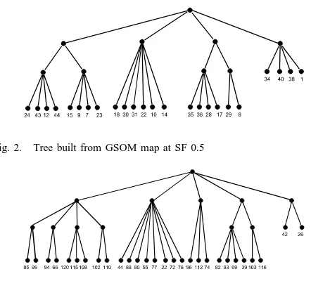
Fig. 2. Tree built from GSOM map at SF 0.5

Fig. 3. Tree built from GSOM map at SF 0.9

IV. EXPERIMENTALRESULTS

A. Data Preparation and Parameter Setting

Zoo data set from UCI machine learning repository [16] is used to demonstrate the concept tree. The GSOM algorithm has been run for 30 iterations for both training and smoothing phases as from the earlier observation, convergence can be achieved before 30th iteration. GSOM algorithm has been run for multiple SFs (high and low spread) to investigate the formation of the tree at different map spread. In the building of the concept tree, threshold for refining clusters at level two is set to 1.5.

B. Evaluation of the Tree from Different SF Values

Different SFs give a different formation of trees as for each SF value, different number of nodes and different weight values will be generated. The first level of the tree is formed by clusters obtained from the cluster identification process. As the lower level will be formed from the upper level, the number of cluster determined in the first level can also have an effect on the formation of the tree. The DB Index values across spread factors from 0.1 to 0.99 are shown in Table I. We show two concept trees with a high and a low SF to compare the effect of the SF value to the tree quality. The concept trees constructed from GSOM map at SF 0.5 and 0.9 are shown in Figures 2 and 3, respectively. These trees are built such that the first layer contains clusters which partition gives the lowest DB index value among theknumber of clusters for a particular SF. As can be seen from the figures, each SF value gives a different structure of tree. There is not much difference in the number of hit nodes between the GSOM maps at SF 0.5 and 0.9 with 24 nodes in SF 0.5 map and 28 nodes in SF 0.9. However, map of SF 0.9 spreads more than SF 0.5 and more detailed nodes have been obtained.

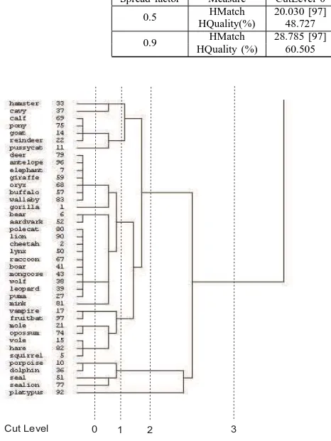
To check the hierarchy quality, we use the hierarchical clustering algorithm (average linkage) to build the target hierarchy. Part of the example output using this algorithm is shown in Figure 4. The hierarchy has been cut into several

levels in order to measure the match at different depth or granularity. Results presented in Table II. For both SF 0.5 and 0.9, the hierarchy quality is increased for the cut towards the upper level of the hierarchy. The result shows that the higher the cut level, more matches in between distinct clusters can be obtained. It is also the ”summarized structure” compared to hierarchical clustering in Figure 4. The similarity of instances between the nodes in the concept tree and the target tree is further observed to confirm the result for the HQuality measure (Table III). The nodes are grouped together according to their parents as shown in Figure 3. It is apparent that most of the nodes have similar animal type and clear separation of the animals can be observed. For example, birds populate node 44, 88, 80, 55, 77, 22, 72 and 76 and the nodes have been combined into a common parent in the tree. Mammals also have been found to be grouped into distinct nodes according to their specific features. For instance, node 85 and 99 consist of mammals which are herbivores whereas node 94 and 66 mostly are carnivorous mammals. Porpoise, dolphin, seal and sealion are grouped together in node 102 and share the same parent with node 110 that contains platypus. Most of the leaf nodes contain instances that are similar to the concept tree’s nodes. At cut level 3, there are four large groups; bird, insect and aquatic animals, aquatic animal together with fish, amphibian and reptile; and lastly mammal. These groups can be found at the first level of the concept tree in Figure 3, for instance, mammals in node 85 to 110 (read from the left to the right side of the tree), birds in node 44 to 76, aquatic animals and fish in node 96 to 74, insects and aquatic animals in node 82 to 116, and finally amphibian and reptiles in node 42 and 26. At cut level 2, more detailed branches have been obtained. Mammals have been separated into three groups with platypus in one; porpoise, dolphin, seal and sealion in one; and all other mammals in another. The mammals are separated further in cut level 1 and 0. At the lower cut, the carnivorous and herbivorous mammals have been separated which is similar to the mammal nodes in the concept tree.

V. CONCLUSIONS

TABLE I

AVERAGE OFDBINDEX VALUES FOR DIFFERENTSFANDk_{= 2}TOk₌√

N₍kIS NUMBER OF CLUSTERS)

k Spread factor

0.1 0.2 0.3 0.4 0.5 0.6 0.7 0.8 0.9 0.99

5 - - - 0.6042 0.5260 0.6066 0.5178 0.5342

4 - - 0.5733 0.5322 0.6549 0.5993 0.5675 0.6303 0.7074 0.5632 3 0.4263 0.7582 0.6479 0.6673 0.6802 0.7399 0.7354 0.7124 0.7567 0.7480 2 0.5396 0.7165 0.7891 0.6934 0.7779 0.8067 0.8328 0.8063 0.7696 0.8240

TABLE II

HIERARCHY MATCH(HMATCH)AND QUALITY OF DISTINCT CLUSTERS(HQUALITY)FOR THE CONCEPT TREES OFSF 0.5ANDSF 0.9. (THE NUMBER IN SQUARE BRACKET IS THE MAXIMUM VALUE FOR THEHMATCH)

Spread factor Measure CutLevel 0 CutLevel 1 CutLevel 2 CutLevel 3

0.5 HMatch 20.030 [97] 15.378 [45] 10.392 [24] 2.588 [6] HQuality(%) 48.727 66.127 79.099 93.105

0.9 HMatch 28.785 [97] 17.462 [45] 11.608 [24] 2.786 [6] HQuality (%) 60.505 68.723 79.631 91.012

0 1 2 3

Cut Level

Fig. 4. The identified mammals group in the hierarchy built using the average linkage algorithm

REFERENCES

[1] T. Kohonen, “The self-organizing map,” Proceedings of the IEEE, vol. 78, no. 9, pp. 1464–1480–, 1990.

[2] D. Alahakoon, S. K. Halgamuge, and B. Srinivasan, “Dynamic self-organizing maps with controlled growth for knowledge discovery,” IEEE Transactions on Neural Networks, vol. 11, no. 3, pp. 601–614, 2000. [3] R. Amarasiri, D. Alahakoon, and K. A. Smith, “Hdgsom: a modified

growing self-organizing map for high dimensional data clustering,” in Fourth international conference on hybrid intelligent, 2004, pp. 216– 221.

[4] N. Ahmad, D. Alahakoon, and R. Chau, “Cluster identification and separation in the growing self-organizing map: application in protein sequence classification,” Neural Computing and Applications, 2009. [5] A. L. Hsu, S.-L. Tang, and S. K. Halgamuge, “An unsupervised

hierar-chical dynamic self-organizing approach to cancer class discovery and marker gene identification in microarray data,” Bioinformatics, vol. 19, no. 16, pp. 2131–2140, 2003.

[6] L. Wickramasinghe and L. Alahakoon, “A novel adaptive decision making agent architecture inspired by human behavior and brain study

TABLE III

NODES AND INSTANCES OF THE CONCEPT TREE FORSF 0.9

Node Number Instances

42 newt, frog

26 slowworm, tuatara, pitviper

103 crab, starfish, crayfish, lobster, clam, octopus

116 scorpion, seawasp 82 flea, worm, slug, termite

93 honeybee, wasp, housefly, gnat, moth

69 ladybird

39 toad

96 catfish, herring, dogfish, pike, bass, pi-ranha, stingray, chub, tuna

112 seasnake

74 seahorse, sole, carp, haddock 44 kiwi, rhea, ostrich

88 wren, parakeet, sparrow, dove, pheas-ant,lark, chicken

80 duck

55 crow, vulture, hawk 77 skua, gull, swan, skimmer

22 tortoise

72 flamingo

76 penguin

85 gorilla, elephant, buffalo, giraffe, oryx, deer, wallaby, antelope

99 goat, reindeer, calf, pony

94 cheetah, bear, pussycat, puma, wolf, leopard, boar, mongoose, lynx, aard-vark, raccoon, polecat, lion

66 mink

120 squirrel, vole, vampire, mole, opossum, hare, fruitbat

115 hamster

108 cavy

102 porpoise, dolphin, seal, sealion

110 platypus

models,” in Fourth International Conference on Hybrid Intelligent Systems, 2004. HIS ’04., Dec. 2004, pp. 142–147.

[7] C.-Y. Chen, Y.-J. Oyang, and H.-F. Juan, “Incremental generation of summarized clustering hierarchy for protein family analysis,” Bioinfor-matics, vol. 20, no. 16, pp. 2586–2596, 2004.

Previous ed.: 2000.

[9] R. S. Michalski, “Knowledge acquisition through conceptual clustering: A theoretical framework and an algorithm for partitioning data into conjunctive concepts,” International Journal of Policy Analysis and Information Systems, vol. 4, pp. 219–244, 1980.

[10] J. W. Tukey, Exploratory Data Analysis. Reading, MA: Addison-Wesley, 1977.

[11] D. S. Moore, The Basic Practice of Statistics, 2nd ed. New York: W. H. Freeman and Company, 2000.

[12] S. Theodoridis and K. Koutroumbas, Pattern recognition, 3rd ed. Am-sterdam ; Boston: Elsevier/Academic Press, 2006, sergios Theodoridis and Konstantinos Koutroumbas.ill. ; 24 cm.Includes bibliographical references and index.

[13] W. M. Rand, “Objective criteria for the evaluation of clustering meth-ods,” Journal of the American Statistical Association, vol. 44, pp. 846– 850, 1971.

[14] P. Jaccard, “tude comparative de la distribution florale dans une portion des alpes et des jura,” Bulletin del la Socit Vaudoise des Sciences Naturelles, vol. 37, pp. 547–579, 1901.

[15] D. H. Widyantoro, “Exploiting homogeneity of density in incremental hierarchical clustering,” in Proceedings of ITB Eng. Science, vol. 39 B, no. 2, 2006, pp. 79–98.