An Extended ID3 Decision Tree Algorithm for Spatial Data

ICSDM2011

Proceedings

2011 IEEE International Conference on Spatial Data

Mining and Geographical Knowledge Services

June 29-July 1, 2011

Fuzhou, China

Editors:

Yee Leung

Chenghu Zhou

Brian

Lees

Diansheng

Guo

Chongcheng Chen

..

+ . I E E E . A

•

Super Map

N S F C

•

An Extended ID3 Decision Tree Algorithm for

Spatial Data

Imas Sukaesih Sitanggang

11

t1

,

Razali Yaakobw

1,

Norwati Mustaphl

3,

Ahmad Ainuddin B Nuruddin·

4

#Faculty of Computer Science and Information Technology, Vniversiti Putra Malaysia 43400 Serdang Selangor, Malaysia

imas. si tanggang@ipb.ac . id; ; razaliy@fsktm. upm. edu.my, Jnorwati@fsktm . upm. edu.my

·1nstitute of Tropical Forestry and Forest Products (INTROP). Universiri Putra Malaysia 43400 Serdang Selangor. Malaysia

•ainuddin@forr.upm.edu.my

tcomputer Science Department. Bogar Agricultural University, Bogar 16680, Indonesia

Abstract-Ulilizing data mining tasks such as classification on spatial data is more complex than those on non-spatial data. It is because spatial data mining algorithms ha ve to consider not only objects or interest Itself but also neighbours of the objects in order to extract useful and Interesting patterns. One or classilication algorithms namely the 103 algorithm which originally designed for a non-spatial dataset bas been Improved by other researchers in the previous work to construe! a spatial decision tree from a spatial dataset containing polygon features only. The objective of this paper is to propose a new spatial decision tree algorithm based on the ID3 algorithm for djscrete features represented in points, lines nod polygons. As in the ID3 algorithm that use information gain in the attribute seleclion, the proposed algorithm uses the spatial information gain to choose the best splitting layer from a set of explanatory layers. The new formula for spatial information gain is propost.'Cl using spatial measures for point, line and polygon features. Empirical result demonslratcs that the proposed algorithm can be used to join

hvo spatial objects in constructing spatial decision trees on small

spatiaJ dataset. The proposed aJgorithm has been applied to the real spatial dataset consisting of point and polygon features. The result is a spatial decision tree with 138 leaves and the accuracy is 74.72%.

Keywords-ID3 algorithm, spatial decision tree, spatiaJ information gain, spatial relation, spatial measure

l. lNTRODUCTION

Utilizing data mining tasks oo a spatial dataset differs with the tasks on 11 non-spntial dataset. Spatial dnta describe

locations of features. ln a non-spatial dataset especially for classification, data arc arranged in a single relation consisting of some columns for attributes and rows representing tuples that have values for each anributes. In a spatiaJ dataset, data are organized in a set of layers representing continue or discrete features. Discrete features include points (e.g. village centres), lines (e.g. rivers) and polygons (e.g. land cover types). One layer relates to other layers to create objects in a spatial dataset by applying spatial relarions such as topological relations and metric relation. Jn spatial data mining tasks we should consider not only objects itself but also their neighbours Lhat could belong to other layers. ln addition, types of attributes in a non-spatial dataset include numerical and categorical meanwhile features in layers are represented by

978-1-4244-83Sl-8/11/S26.00 ©2011 IEEE

geometric types (polygons, lines or points) that have quantitative measurements such as area and distance.

This paper proposes a spatial decision tree algorithm 10

construct a classification model from a spatial dataset. The dataset contains only discrete features: points, lines and polygons. The algorithm is an extension of ID3 algorithm [I) for a non-spatial dataset. As in rhe ID3 algorithm, the proposed algorithm uses information gain for spatial data, namely spatial infonnation gain, to choose a layer as a splitting layer. Instead of using nwnber of tuples in a partition, spatial information gain is calculated using spatial measures. We adopt the fomiula for spatial infonnation gain proposed in [2). We extend the spatial measure definition for the geometry type points, lines and polygons rather than only for polygons as in [2].

The paper is organized as follows: introduction is in section 1 . Related works in developing spatial decision tree algorithms are briefly explained in section 2. Section 3 discusses spatia.1 relationships. We explain a proposed spatial decision tree algorithm in section 4. Finally we summarize the conclusion in section 5.

ll. RELATED WORKS

The works in developing spatial data mining algorithms including spatial classification and spatial association rules continue growing in recent years. The discovery processes such as classification and association rules mining for spatial data are more complex than those for non-spatial data, because spatial data mining algorithms have to consider the neighbours of objects in order to extract useful knowledge (3).

In tbe spatial data mining system, the attributes of the neighbours of an object may have a significant influence on the object itself.

classified but to consider also attributes of neighbouring objects. The algorithm docs not make distinction between thematic layers and it takes into account only one spatial relationship [4]. The decision tree from spatial data was also proposed as in [5]. The approach for spatial classification used in (5) is based on both (I) non-spatial properties of the classified objects and (2) attributes, predicates and functions describing spatial relation between classified objects and other features located in the spatial proximity of the classified objects. Reference [ 6) discusses another spatial decision tree algorithm namely SCART (Spatial Classification and Regression Trees) as an extension of Lhe CART method. The CART (Clnssification and Regression Trees) is one of most commonly used systems for induction of decision trees for classification proposed by Briemnn et. al. in 1984. The SCART considers the geographical data organized in thematic layers, and their spatial relationships. To calculate the spatial relationship between the locations of two collections of spatial objects, SCART has the Spatial Join Lndex (SJI) table [7] as

one of input parameters. The study [2] extended the 103 algorithm [I] such that the new algorithm can create

a

spatial decision rree from the spatial dataset talcing into account not only spatial objects itself but also their relationship to its neighbour objects. The algorithm generates a tree by selecting the best layer to separate a dataset into smaller panitions as pure as possible meanmg that all tuples in panitions belong to the same class. As in the lD3 algorithm, the algorithm uses the information gain for spatial data, namely spatial information gain, to choose a layer as a splitting layer. Instead of using number of tuples in a panition, spatial information gain is calculated using spatial measures namely area [2].

lll. SPATIAL RELATIONSlllP

Determining spatial relationships between two features is a

major function of a Geographical Information Systems (GISs). Spatial relationships include topologicaJ [8] such as overlap, touch, and imersect and metric such as distance. For example, two different polygon features can overlap, touch, or intersect

each other. Spatial relationships make spatial data mining

algorithms differ from non-spatial data mining algorithms. Spatial relationships are materialized by an extension of the well-known join indices [7]. The concept of join index between two relations was proposed in [9). The result of join mdex between two relations is a new relation consisting of indices pairs each referencing a tuple of each relation. The pairs of indices refer to objects that meet the join criterion. Reference f7] introduced the structure Spatial Join Index (SJI) as an extended the join indices (9] in the relational database framework. Join indices can be bandied in the same way than other tables and manipulated using the powerful and the standardized SQL query language (7). It pre-computes the exact spatial relationships between objects from thematic layers [7). Ln addition, a spatial join index has a third column that contains spatial relationship, SpatRel, between two layers. Our study adopts the concept of SJI as in [7] to store the relarions between rwo different layers in spatial database. Instead of spatial relationship that can be numerical or

Boolean value, the quantjtative values in the third column of SJI are spatial measure of features as results from spatial relationships between two layers.

We consider an input for the algorithm a spatial database as

a set of layers L. Each layer in L is a collection of geographical objects and has only one geometric type that can be polygons, or lines or points. Assume that each object of

a

layer is uniquely identified. Let L is a set of layers, L1 and Lj are two distinct layers io L. A spatial relationship applied to L1 and L, is denoted SpatRel(Lu L₁) that can be topological

relation or metric relat100. For the case of topological relation, SpatRol{L_1, Lj ) is a relation according to the dimension extended method proposed by [I 0). While for the case of metric relation, SpatRel(oi. o,) is a distance relation proposed by [ 11 ], where o; is a spatial object in L, and o, is a spatial object in L,.

Relations between two layers in a spatial database can

result quantitative values such as distance between two points or intersection area of two polygons in each layer. We denote these values as spatial measures as in [2] that will be used in calculating spatiaJ infonnation gain in the proposed algorithm. For the case of topological relation, the spatial measure of a feature is defined as follows. Let L1 and L, in a set of layers L, L, -f. L,, for each feature r; in R = SpntRel(L,, L,), a spatial measure of r, denoted by SpatMes(r,) is defined as

I. Arca of r11 if< L., in, LJ >or< L,, overlap, L1 >hold for

all features in L_{1 and} L, represented in polygon

2. Count of r., if < L., in, L, > bolds for all features m L, represented in point and all features in L, represented in polygon.

For the case of metric relation, we define a distance function from p to q as dist(p, q), distance from a point (or line) pin L, to a point (or line) q in Lt

Spatial measure of R is denoted by SpatMcr(R) and defined as SpatMcs(R)"" f(SpatMes(r1) , SpatMes(r2), .. • , SpatMes(rn))

(1)

for r, in R, i = I, 2, ... , n and n number of features in R. f is an aggregate function that can be sum, min, max or average.

A spatial relationship applied to

Li

and Lj in L results a new layer R. We define a spatial join relation (SJR) for aJJ features

p in L, and q in L, as follows:

SJR = {(p, SpatMcs(r), q Ir is a feature in R associated top

and q}. (2)

IV. EXTENDED lD3 ALGORITHM FOR SPATIAL DATA

(polygons, lines or points) in the target layer are related to features in explanatory layers to create a set of tuples in which each value in a tuple corresponds to value of these layers. Two distinct layers are associated to produce a new layer using a spatial relationship. Relation between two layers produces

a

spalial measure (l)

for the new

layer. Spatial measure then will be used in the formuJa for spatial infonnation gain.

Building a spatial decision tree follows the basic leaming process in the algorithm ID3 [I). The ID3 calcuJates information gain to define the best splitting layer for the dataset. ln spatial decision tree algorithm we define the spatial infonnation gain to select an explanatory layer L that gives best splitting the spatial dataset according to values of predictive attribute in the layer L. For this purpose, we adopt the fonnula for spatial infonnation gain as in [2) and apply the spatial measure ( 1) to the formula.

Let a dataset D be a training set of class-labelled tuples. lo the non-spatial decision tree algorithm we calculate probability that an arbitrary tuples in D belong to class Ci and it is estimated by

ICi.01/IDI

where

IDI

is number of tuples in D and

IC;,ol

is number of tuples of class

Ci

in

D [

12]. lo this study, a dataset contains some layers including a target layer that store class labels. Number of tuples in the dataset is the same as number of objects in the target layer because each tuple will be created by relating features in the target layer to features in explanatory layers. One feature in the target layer will exactly associate with one tuple in the dataset. For simplicity we will use number of objects in the target layer instead of using number of tuples in the spatial dataset. Furthennore in a non-spatial dataset, target classes arc discrete-valued and unordered (categoric:il) and explanatory attributes are categorical or numerical. Jn spatial dataset, features in layers are represented by geometric type (polygons, lines or points) that have quantitative measurements such as

area and distance. For that we calculate spatial measures of Layers (I) to replace number of tuples in a non-spatial data partition.

A . Entropy

Let a target attribute C in a target layer S has I distinct classes (i.e. Ci. c2, ... , c1), entropy for S represents the

expected infonnation needed to determine the class of tup.les in the dataset and defined as

ｾ＠ SpatMes(Se) SpatMes(Sc )

H(S) = -£...,, ' log2 ' (3)

;,.1 SpatMes(S) SpatMes(S)

SpatMes(S) represents the spatial measure of layer S as defined in (I).

Let an explanatory attribute V in an explanatory (non-target) layer L bas q distinct values (i.e. v1, v2, ... , vq). We partition

the objects in target layer S accordfag to the layer L then we have a set of layers L(v;, $)for each possible value v, in L. In our work, we asswne that the layer L covers all areas in the layer S. The expected entropy value for splitting is given by:

ｾ＠ SpatMes(L(v . S))

H(S I L)=

L

1' H(L(v .,S)) (4)

j•I SpatMes(S) 1

H(SJL) represents the amount of information needed (after the partitioning) in order to arrive at an exact classification.

8. Spatial Information Gain

The spatial information gain for the layer Lis given by: Gain(L) = H(S) - H(SIL) (5)

Gain(L) denotes how much infomrntion would be gained by branching on the layer L. The layer L with the highest infonnation gain, (Gain(L)), is chosen as the splitting layer at a node N. This is equivalent to say that we want to partition objects according to layer L that would do the "best classification", such that the amount of information still required to complete classifying the objects is minimal (i.e., minimum H(SIL)).

C. Spatial Decision Tree Algorithm

fig. I shows our proposed algorithm to generate spatial decision tree (SOT). Input of the algorithm is divided into two groups: I) a set of layers containing some explanatory layers and one target layer that bold class labels for tuples in the dataset, and 2) spatial join relations (SJRs) storing spatial measures for features resulted from spatial relations bet\veen two layers. The algorithm generates a tree by selecting the best layer to separate dataset into smaUer partitions as pure as

possible meaning that all tuples in partitions belong to the same class.

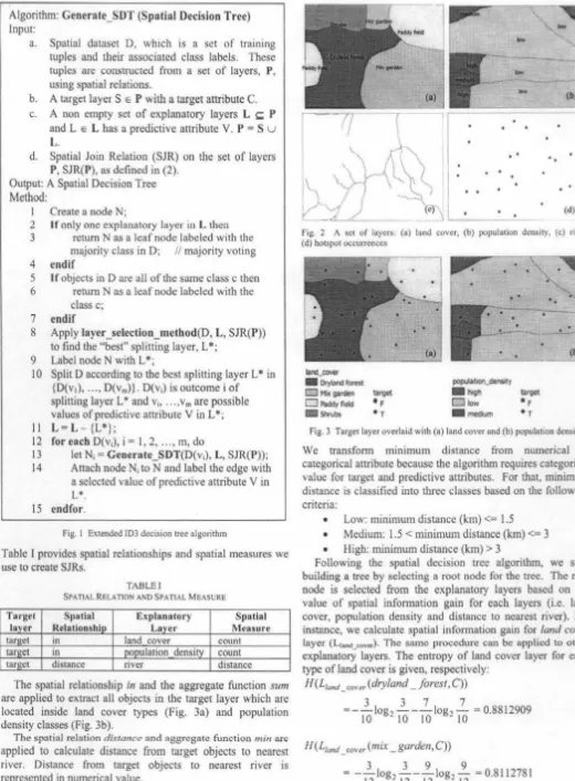
To illustrate how the algorithm works, consider an active fire dataset containing three explanatory layers: land cover (Lrond_covcr), population density (Lpopul•uoo_dciiso1y) and river (Lmcr), and one target layer (Lt.arg<i) (Fig. 2).

Land cover layer represents polygon features for land cover

types. It has a predictive attribute that contains land cover types in the study area. They are dryland forest, paddy field, mix garden, shrubs, and paddy field (Fig. 2a).

Population layer contains polygon features for population density. The layer bas a predictive attribute population class

representing classes for population density (Fig. 2b). Classes for popuJatfon density are as follows :

• Low: population_ density <= 50

• Medium: 50 < population_ density <= 150 • High: population_ density> 150

River layer bas only two attribulcs: the identifier of objects and geometry representation for lines.

Target layer represents point features for true and false alann. True alarms

Cn

arc active fires (hotspots) and false alarms (F) are random points generated near true alarms.

The algorithm requires spatial measures in the spatial join relation (SJR) between lhe target layer and an explanatory

Algorithm: Generate_SDT (Spatial Decision Tree)

Input:

a. Spatial dataset D, which is a set of training tuples and their associated class labels. These tuples arc constructed from a set of layers, P,

using spatial relations.

b. A target layer S e P with a target attribute C.

c. A non empty set of explanatory layers L ｾ＠ P and L e L has a predictive attribute V. P =Su

L.

d. Spatial Join Relation (SJR) on the set of layers P, SJR(P), as defined in (2).

Output: A Spatial Decision Tree

Method:

I Create a node N;

2 If only one explanatory laye1 in L then

3 return N as a leaf node labeled with the majority class in D; II majority voting

4 endif

5 If objects in Dare all of the same class c then

6 return N as a leaf node labeled with the class c;

7 endif

8 Apply layer_selection_mcthod(D, L, SJR(P)) to find the "best" splitting layer, L •;

9 Label node N with L*;

I 0 Split D according to the best splitting layer L • in {D{v1) •... , D(v ... )}. D(v,) is outcome i of splitting layer L• and v,, ... ,Vm are possible

values of predictive aetributc V in L *;

II L = L - {L*};

12 for each D(v,), i = 1, 2, ... , m, do

13 let N1 ... Generate_S DT(D{v,), L, SJR(P));

14 Attach node N, to N and label the edge with a selected value of predictive attribute V in L*

15 endfor.

Fig 1 Extended ID3 decision 1rcc nlgorithm

Table I provides spatial relationships and spatial measures we use to create SJRs.

TABLEl

SPATIAL RFLATION Al'OSPATIAL MEASURE

T argec Sp1Ulal Explanatory Spatial

layer Relationshio Layer Measure

tar1?et in land cover count

1araet m oooulation density count target distance ri\<er distance

The spatial relationship in and the aggregate function sum

are applied to extract all objects in the target layer which arc located inside land cover types (Fig. 3a) and population density classes (Fig. 3b).

The spatial relntion tlfrumce and asgrcgatc function min arc

applied to calculate distance from target objects to nearest river. Distance from target objects to nearest river is represented in numerical value.

Fig. 2 /\ sec of layers: (o) land cover, (b) population dcrn;11y, (c) nver.

(d) hotspot occurrences

tancl_COYer • Oryland fonllt

D ＢＧｾ＠ 91tc1tn tat9't

0 Paddy fltld ' F • strubs • T

popjAOon_denslty

• ｾｨ＠ taroel

Dlow • F

• medum • T

Fig. 3 Targc1 layer overlaid with (a) lnnd cover nnd (b) population density

We transfonn minimum distance from numerical to categorical attribute because the algonthm requires categoncal value for target and predictive attributes. For that, minimum distance is classified into three ｣ｬ｡ｳｾ｣ｳ＠ based on the following criteria:

• Low: minimum distance (km)<= 1.5 • Medium: 1.5 < minimum distance (km) <= 3 • High: minimum distance (km)> 3

Following the spatial decision tree algorithm, we start building a tree by selecting a root node for the tree. The root node is selected from the explanatory layers based on the value of spatial infonnatioo gain for each layers (i.e. land cover, population density and distance to nearest river). For instance, we calculate spatial infonnation gain for land cover

layer ( L1anc1 co_). The same procedure can be applied to other

explanatory layers. The entropy of land cover layer for each type of land cover is given, respectively:

H(L1und_cov,.,.(dryland _foresr.C))

3 3 7 7

•-iOlog2 i0-i0log2 iO = 0.8812909

11 (llund mtr (mll: _garden, C))

3 3 9 9

[image:5.620.21.541.8.714.2]

-H(Lfand ｟｣ｯｾｲＨｐ｡､､ｹ＠ _jield,C))

6

6 0

0

-=

-6log2 6-6

log2

6

= O

H(l1unJ _coHr(Shrubs,C))

0 0 2 2

=

-2log22-21og2

2"

=O

From (4) we calculate the expected entropy value for splitting:

H(S

I

L/unJ _com)

］ｾｸＰＮＸＸＱＲＹＰＹＫ＠

12

x0.8 112781

ＫｾｸｯＫＲＭｸｯ＠

30 30 30 30

=

0.618274883 Entropy for the target layer S:

12 12 18 18 H(S) =

-30 log2 30 - 30 log2 30 = 0.970950594 From (5) we calculate the information gain for land cover

layer:

Gain(Lland co•n) = H(S) - I l(SIL'-1 ..,,.,) = 0.352675712 The spatial information gam for other layers is as follows

Gain(L.,op..1Mion_c1nu.1y)

=

0.18538127 Gain(Lmn)

=

0.097717695

ｾ＠ foroat , ,,.,.. Mix

,. gardon

/:

LON Medun

｜ ｾ＠

GG

8

4.

5.

Fig. 4 Spatial decision tree

IF land cover is mix garden AND distance to nearest river is low THEN Hotspot Occurrence is True

IF land cover is mix garden AND distance to nearest river

is medium THEN Hotspot Occurrence is True

ｌＱ｡ｮ､ ｟｣ｯｶ ｾ＠ has the highest spatial infonnation gain compared to

two other layers. Therefore Lland covn

is

selected as the root of 6.

the tree. There are four possible-values for land cover types: dryland forest, mix garden, paddy field, and shrubs that will 7.

IF land cover is mix garden AND distance 10 nearest river

is high THEN Hotspot Occurrence 1s False

IF land cover is paddy field THEN Hotspot Occurrence is False

be assigned as label of edges connecting the root node to internal nodes.

The Gcnerate_SDT algorithm is then applied to a set of layer containing new explanatory layers and the target layer to construct a subtree attached to the root node. New explanatory layers arc created from existing explanatory layers, best layer and the value vj of predictive attribute as a selection criterion in a query to relate an explanatory layer and the best layer. The tree will stop growing if it meets one of the following termination criteria:

l. Only one explanatory layer in L. In this situation, the algorithm returns a leaf node labeled with the majority class in the SJR for the best layer and the explanatory layer.

2. The SJR for best layer and explanatory layer contains the same class c. Theo the algorithm returns a leaf node labeled with the closs c.

The graphical depictjon of spatial decision tree generated from P

=

{L1anc1_co,a, ｬｰｯｰＮＮＱＮＱｩｯｮ ｟ｾ ＱＱｹＮ＠ Lmm target (S)} is shown in Fig. 4. The final spatial decision tree contains 8 leaves and

3 nodes with the ftrst test attribute is land cover (Fig. 4).

Below are rules extracted from the tree:

I. IF land cover is dryland forest AND population density is low Tl IEN Hotspot Occurrence is True

2. IF land cover is dryland forest AND population density is medium THEN Hotspot Occurrence is True

3. IF land cover is dryland forest AND population density is high THEN Hotspot Occurrence is False

8. IF land cover is shrubs THEN Hotspot Occurrence is True

The decision tree has the misclassification error of the training set: 16.67% and the error of the testing set: 20%. The accuracy of the tree on the testing set is 80%. The number of target objects in the testing set is 30 and the number of correctly classified objects is 24.

The proposed algorithm bas been applied to the real active fires dataset for the Rokan Hilir District. Riau Province Indonesia with the total area is 896, 142.93 ha. The dataset contains five explanatory layers and one target layer. The target layer consists of active fires (hotspots) as trne alarm data and non-hotspots as false alarm data randomly generated near hotspots. Explanatory layers include distance from target objects to nearest river {dist_river), distance from target objects to nearest road (dist_road), land cover, income source and population density for the village level in the Rokan Hilir District. Tabet II summaries the number of features in the dataset for each layer.

TABLE Ill

NU\1BER OF FEA TUR.ES IN TIIE DATASET

La er dist river

dist road

•

The decision tree generated from the proposed spatial decision tree algorithm contains 138 leaves with the first test attribute is distance from target objects to nearest river (dist_ river). The accuracy of the tree on the training set is 74.72% in which 182 of 720 target objects arc incorrectly classified by the tree. Some preprocessing tasks will be applied to the real spatial dataset such as smoothing to remove noise from the data, discretization and ggeneralization in order to obtain a spatial decision tree with the higher accuracy.

V. CONCLUSIONS

This paper presents

an extended 103 algorithm that can be

applied to a spatial database containing discrete features (polygons, lines and points). Spatial data are organized in a set of layers that can be grouped into two categories i.e. explanatory layers and target layer. Two different layers in the database are related using topological relationships or metric relationship (distance). Quantitative measures such as area and distance from relations between two layers are then used in calculating spatial information gain. The algorithm will select an explanatory layer with the highest information gain as the best splitting layer. This layer separates the dataset into smaller partitions as pure as possible such that all tuples in partitions belong to the same class.

Empirical result shows that the algoritlun can be used to join two spatial objects in constructing spatial decision trees on small spatial dataset. Applying the proposed algorithm on the real spatial dataset results a spatial decision tree containing 138 leaves and the accuracy of the tree on the training set is 74.72%.

ACKNOWLEDGMENT

The authors would like to thank Indonesia Directorate General of Higber Education (IDGHE), Ministry of National

Education, Indonesia for supponing

PhD

Scholarship (Contract No. 1724.2/04.4/2008) and Southeast Asian Regional Centre for Graduate Study and Research in Agriculture (SEARCA) for partially supporting the research.

REFERENCES

[I) J. R. Quinlan, "Induction of Decision Trees," Machine learning, vol. I,

Kluwer Academic Publishers, Boston, pp. 81-106, 1986.

(2) S. Rini.ivillo and T. Franco, Classificotion in Geographical

Information Systems. Lecture Notes in Artificial Intelligence. Berlin

Heidelberg: Springer-Verlag, pp. 374-385. 2004.

[3) .M. Ester, Kr. I lans-Pctcr. and S. Jorg, "Spatial Daill Mining. /\

Database Approach," in Proc. of the Fifth Int. Symposmm on Large

Spatial Databases, Berlin, Germany, 1997.

l4) K. Zc1touni and C. Nadjim, ''Spatial Decision Tree - Application to

Traffic Risk Analysis," in ACS/IEEE lfllemational Co11fere11ce, IEEE,

2001.

LS) K. Koperski, J. Han and N. Stefanovic, .. An efficient two-step method

for classification of spatial data," In Symposium on Spatial Datu

llandling, 1998.

[6) N. Chclghoum, Z. Karine, and B. Azcdinc, "A Decision Tree for

Multi-Layercd Spatial Data,'' in Sympusium on Geo.1pc11ial T11eory.

Processing and Applicatio11s, Ottawa, 2002.

[7) K. Zeitouni. L. Yeh, a11d M.A. Aufaure, "Join Indices as a Tool for

Spatial Data Mining," in lmernational Work.rhop 011 Temporal. Spmial

and Spatio· Temporal Data Mining, 2000.

[8] M. J. Egenhofer, and D. F. Roben, "Point-set topological spatial

relations," lntemational Journal of Geograpl11cul lnfannation Systems,

vol.5(2), pp. 161 - 174,1991.

(9] P. Valduriei, "Join indices," ACM Trans. on Database Systems, vol.

12(2), pp. 218-246, June 1987.

[10] E. Clcmentiol, P. Di Felice, and 0. Oosterorn, A small set of formal

topological relation.rhips suitable for end-user interaction. Lecture Notes in Computer Science. New York: Springer, pp. 277- 295, 1993. (11] M. Ester, K. Huns-Peter, and S. JOrg, "Algorithms nnd Applications for

Spatial Data Mining," Geographic Data Minmg and Knowledge

Disco1•ery. Research Monographs in GIS, Taylor and Francis, 2001.

[ 12] J. llan and M. Kamber. Data Mimng Concepts and Tec/1111que.s. 2nd