Variance
Song S. Qian
∗Zehao Shen
†April 9, 2007
Abstract 1
A Bayesian representation of the analysis of variance by Gelman (2005) is 2
introduced with ecological examples. These examples demonstrate typical 3
situations we encounter in ecological studies. Compared to the conventional 4
methods, the multilevel approach is more flexible in model formulation, easier 5
to setup, and easier to present. Because the emphasis is on estimation, 6
multilevel model results are more informative than the results from a 7
significance test. The improved capacity is largely due to the changed 8
computation methods. In our examples, we show that (1) the multilevel 9
model is able to discern a treatment effect that is too weak for the 10
conventional approach, (2) the graphical presentation associated with the 11
multilevel method is more informative, and (3) the multilevel model can 12
incorporate all sources of uncertainty to accurately describe the true 13
relationship between the outcome and potential predictors. 14
∗Corresponding author, phone 919 613-8105, email: [email protected], Nicholas School of the
En-vironment and Earth Sciences, Duke University Durham, NC, USA
†Department of Ecology, College of Environment Science, Peking University, Beijing, China
Key terms: ANCOVA, ANOVA, Bayesian statistics, hierarchical model,
Analysis of variance (ANOVA) is widely used in scientific research for testing
18
complicated multiple hypotheses. As presented originally in Fisher’s seminal work
19
(Fisher, 1925), ANOVA can be seen as the collection of the calculus of sum of
20
squares and the associated models and significance tests. These tests and models
21
have had a profound impact on ecological studies. ANOVA provides the
22
computational framework for the design and analysis of ecological experiments
23
(Underwood, 1997). As a data analysis tool, ANOVA is used in ecology for both
24
confirmative and explorative studies. When used in a confirmative study, the
25
randomized experimental design ensures that the resulting difference between
26
treatments can be unambiguously attributed to the cause we are interested in
27
testing. When used in explorative studies, the ANOVA framework reflects a basic
28
scientific belief that correlation implies a causal relationship (Shipley, 2000). The
29
simple steps of ANOVA computation, along with the associated significance test
30
(the F-test), allow quick implementation and seemingly straightforward
31
interpretation of the results.
32
Interpretation of ANOVA results can be problematic. Difficulties arise when the
33
normality and independence of the response data are not met, when the
34
experimental design is nested, when using an unbalanced design, or when missing
35
cells are present. More importantly, ANOVA results are difficult to explain in
36
ecological terms because significance test results are usually not scientifically very
37
informative (Anderson et al., 2000). On one hand, when an experiment is proposed,
we almost always have reasons to believe that a treatment effect exists. Therefore,
39
we want to know the strength of the effect a treatment has on the outcome rather
40
than whether the treatment has an effect on the outcome. By using a significance
41
test basing the inference on the assumption of no treatment effect, we emphasize the
42
type I error rate (erroneously reject the null hypothesis of no treatment effect) often
43
at the expense of statistical power, especially when multiple comparison is used. On
44
the other hand, a nonexistent treatment effect can be shown to be statistically
45
significant if one tries often enough (hence the article by Ioannidis, 2005).
46
From this practical perspective, we find the concept of variance components (Searle
47
et al., 1992) especially useful. The relative sizes of the two variances indicate the
48
effects of the factors of interest. When graphically presented, this partitioning of
49
total variance into compartments is actually more informative than the results of a
50
significance test. The ambiguity and difficulty of ANOVA can be alleviated by using
51
a multilevel (or hierarchical) modeling approach for ANOVA proposed by Gelman
52
(2005). His method can be summarized as the estimation of the variance
53
components and treatment effects using a hierarchical regression. The results are
54
often presented graphically. This approach is intuitively appealing and its
55
implementation is straightforward even when the experimental design is nested and
56
the response variable is not normally distributed. The multilevel ANOVA is
57
Bayesian and inference about treatment effects are made using Bayesian posterior
58
distributions of the parameters of interest. Gelman and Tuerlinckx (2000) suggested
59
that the hierarchical Bayesian approach for ANOVA includes the classical ANOVA
60
as a special case. We introduce Gelman’s multilevel ANOVA using three examples.
61
Statistical background are presented in Gelman (2005), Gelman and Hill (2007),
62
and Gelman and Tuerlinckx (2000), and are briefly discussed in the supplementary
63
materials.
2
Methods
65
We illustrate the multilevel ANOVA approach using a one-way ANOVA setting. For
66
a one-way ANOVA problem, we have a treatment with several levels, and the
67
statistical model is:
68
yij =β0 +βi+ǫij. (1)
69
where β0 is the overall mean,βi is the treatment effect for level i and
P
βi = 0, and
70
j represents individual observations in treatment i. This is a multilevel problem
71
because we are interested in parameters at two levels: the data level and the
72
treatment level. At the data level, individual response variable values are governed
73
by the group level parameters, and the group level parameters are further governed
74
by a distribution with hyper-parameters. The term “multilevel” is used to describe
75
the data structure (data points are clustered in multiple treatment levels) and the
76
hierarchical model structure. We avoid the usually used terms “fixed” or “random”
77
effects to avoid confusion as described in Gelman and Hill (2007, sections 1.1 and
78
11.4) and Gelman (2005, section 6). The term “multilevel” encompasses both fixed
79
and random effects. The total variance in yij is partitioned into between group
80
variance (var(βi)) and within group variance (var(ǫij)). Instead of using the
81
sum-of-squares calculation, we use a hierarchical formulation and model the
82
coefficients βi as a sample from a normal distribution with mean 0 and varianceσ
2
The model error term ǫij is also modeled as from a normal distribution:
The variance component for the treatment can be naturally estimated by σβ, or the
89
standard deviation of ˆβi (sβ, the finite population standard deviation). The
90
computation expressed here is standard for random effect coefficients under classical
91
random effect model (Clayton, 1996). We can view fixed effects as special cases of
92
random effects (σβ =∞) in a Bayesian context. Therefore, this computation
93
framework is not unique for Bayesian.
94
Model coefficients (β’s and σβ, orsβ can be estimated using the maximum likelihood
95
estimator, and the likelihood function of this setting is a product of two normal
96
distribution density functions defined by equations 1 and 2. Analytical solutions are
97
often available, but it is easy to implement the computation using Markov chain
98
Monte Carlo simulation (MCMC, Gilks et al., 1997; Qian et al., 2003).
99
When there is more than one factor affecting the outcome, we can easily extend the
100
approach by using the same hierarchical representation of the additional factors.
101
Furthermore, as suggested by equation 3, this approach is not limited by the
102
normality assumption. That is, the normal distribution in equation 3 can be
103
replaced with any distribution from the exponential family, similar to the
104
generalization from linear models to the generalized linear models (GLM,
105
McCullagh and Nelder, 1989).
106
2.1
Data Sets and Models
107We illustrate the multilevel ANOVA using three data sets. The intertidal seaweed
108
grazers example, a textbook example of ANOVA, is intended to make a direct
109
comparison between the multilevel ANOVA and the classical ANOVA. The
110
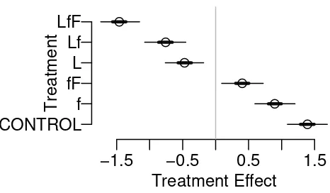
Liverpool moths example is used to illustrate the application of multilevel model
111
under a logistic regression setting, where the response variable follows a binomial
distribution. The seedling recruitment data set illustrates the use of this approach
113
for count data (Poisson regression) that may be spatially correlated. Results from
114
applying the classical ANOVA or linear modeling are presented in the
115
Supplementary Materials.
116
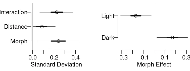
2.1.1 Intertidal Seaweed Grazers
117
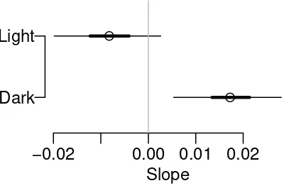
This example was used in the text by Ramsey and Schafer (2002) (Case Study 13.1,
118
p. 375), describing a randomized experiment designed to study the influence of three
119
ocean grazers, small fish (f), large fish (F), and limpets (L), on regeneration rate of 120
seaweed in the intertidal zone of the Oregon coast. The experiments were carried
121
out in eight locations to cover a wide range of tidal conditions and six treatments
122
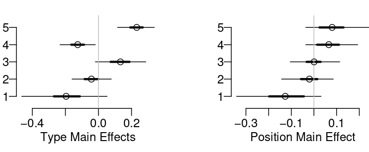
were used to determine the effect of different grazers (C: control, no grazer allowed; 123
L: only limpets are allowed; f: only small fish allowed; Lf: large fish excluded; fF: 124
limpets excluded; and LfF: all allowed). The response variable is the seaweed
125
recovery of the experimental plot, measured as percent of the plot covered by
126
regenerated seaweed. The standard approach illustrated in Ramsey and Schafer
127
(2002) is a two-way ANOVA (plus the interaction effect) on the logit transformed
128
percent regeneration rates. The logit of percent regeneration rate is the logarithm of
129
regeneration ratio (% regenerated over % not regenerated).
130
Using the multilevel notation, this two-way ANOVA model can be expressed as:
131
interaction effect (Pβ3ij = 0). The residual term ǫijk is assumed to have a normal
135
distribution with mean 0 and a constant variance, where k = 1,2 is the index of
individual observations within each Block – Treatment cell. The total variance in Y
137
is partitioned into four components: treatment, block, interaction effects, and
138
residual.
139
2.1.2 Liverpool Moths
140
Bishop (1972) reported a randomized experimental study on natural selection. The
141
experiment was designed to answer the question that whether blackened tree trunks
142
by air pollution near Liverpool, England were the cause of the increase of a dark
143
morph of a local moth. The moths in question are nocturnal, resting during the day
144
on tree trunks. In Liverpool, a high percentage of the moths are of a dark morph,
145
whereas a higher percentage of the typical (pepper-and-salt) morph are observed in
146
the Welsh countryside, where tree trunks are lighter. Bishop selected seven
147
locations progressively farther away from Liverpool. At each location, Bishop chose
148
eight trees at random. Equal numbers of dead light and dark moths were glued to
149
the trunks in lifelike positions. After 24 hours, a count was taken of the numbers of
150
each morph that had been removed – presumably by predators. The original study
151
was published before the time of GLM, but the data set has since been used in
152
several regression textbooks as an example of logistic regression (e.g., Ramsey and
153
Schafer, 2002). We choose to model the moth data as from a binomial distribution
154
and use the typical logistic regression model:
155
the jth distance (distance from Liverpool),nij is the total number of moths placed
158
on each tree,pij, the parameter of interest, is the probability a moth being removed,
159
β1i is the morph effect, and β2i is the slope on distance, representing the interaction
between morph color and distance. Bishop (1972) and Ramsey and Schafer (2002)
161
used a categorical predictor “site” instead of distance from Liverpool to account for
162
the apparent outlier at distance of 30.2 km (Figure 3 of the supplementary
163
materials). We choose to use distance as a continuous predictor to illustrate the
164
interaction effect between a categorical predictor and a continuous predictor.
165
2.1.3 Seedling Recruitment
166
Shen (2002) reported an observational study on factors affecting the species
167
composition and diversity of a mixed evergreen-deciduous forest community in
168
southwest China. The original study has observations at multiple spatial scales. We
169
use the seedling recruitment data collected along a transect of 128 5×5 meter
170
consecutive plots to study factors affecting seedling recruitment. A total of 49
171
species of seedlings were observed in the field and were classified into 5 types
172
according to their status in community dynamics (Shen et al., 2000): Pioneer, Early
173
dominant, Early companion, Later dominant (including evergreen species), and
174
Tolerant. Within each plot, number of seedlings (height below 1 meter) was
175
recorded, along with several physical and biological variables, including canopy gap
176
measured in % (Gap), position of each plot measured as relative position along a
177
hillside between valley (P osition= 1) and ridge (P osition= 5), soil total organic
178
carbon (T OC, in %).
179
The observed number of seedlings (the response variable) from different plots are
180
likely correlated, and the correlation is likely due to the spatial layout of the
181
transect. A natural strategy for this problem is to introduce a spatial random
182
effects term ǫ using the intrinsic conditional autoregressive model (CAR) (Besag et
al., 1991; Qian et al., 2005):
position, l is the index of observations within a plot. The spatial random effect term
187
ǫi has a CAR prior. It is used to model the spatially structured variation. The error
188
term εi is used to account for unstructured over-dispersion. The sum of ǫi and εi is
189
termed as the convolution prior (Besag et al., 1991). Only two-way interactions
190
between T ype and the two continuous predictors were considered.
191
3
Results
192
Results from using classical approach are presented in the supplementary materials.
193
All multilevel results are presented graphically, showing the estimated posterior
194
mean (the circle), the 50% (thick line) and 95% (thin line) posterior credible
195
intervals. The ANOVA display shows the estimated posterior distributions of
196
variance components (in standard deviation), and the effects plots are based on
197
estimated posterior distributions of effects.
198
3.1
Seaweed Grazers
199The multilevel model results are qualitatively similar to the conventional ANOVA
200
results (Figure 1). In addition, the estimated main effects are similar to results from
201
a conventional ANOVA (Figures 2 and 3). The emphasis on estimation is clearly
202
displayed in these plots. From the main effects plots, we know that the maximum
203
difference between treatment and control is about 3 in logit scale, or the mean
204
regeneration ratio of the control sites is about 20 times (e3
) larger than that of the
treatment Lf F sites. Traditional ANOVA does not emphasize the interaction effect
206
beyond whether or not it is statistically significant. See supplementary materials for
207
a comparison of the multilevel interaction plot and the commonly used interaction
208
plot in ANOVA.
209
3.2
Moths
210Using the multilevel model, we can use the traditional analysis of covariance
211
(ANCOVA) setup to calculate the variance components of the main morph effect,
212
main distance effect and the interaction (Figures 4-5). For this particular example,
213
we see a strong interaction effect (clearly expressed by the difference in the
214
distance slope in Figure 5) and an unambiguous morph main effect (Figure 4 right 215
panel). The morph main effect is obvious because it is evaluated at a distance of
216
27.2 (the average distance).
217
3.3
Seedling Recruitment
218The largest variance component is the unstructured over-dispersion term, while the
219
structured spatial random effects (CAR) contributes a smaller than expected
220
variance (Figure 6). The inclusion of spatially correlated predictors may have
221
accounted for some spatial autocorrelation in the response variable data. The
222
variableT ypeexplains the most variation in recruitment (Figures 6 and 7 left panel),
223
which is expected since tree species were classified to reflect their different ecological
224
strategies and roles in community dynamics. Similar to the GLM results, we found
225
the effect of GAP is uncertain. However, the T ype:GAP interaction effect, as
226
shown in terms of type-specific GAP slope (Figure 8, right panel), indicates that
227
type 4 (late dominant) trees are likely to respond negatively to increased gap, while
the rest likely respond positively. The interaction effect between T ype and T OC
229
(Figure 8, left panel) is unambiguous. Because soil carbon concentration is likely to
230
be similar in neighboring plots, including a spatial autocorrelation term reduces
231
uncertainty on type-specific T OC slopes. Type 4 and 5 trees include all evergreen
232
species and the shade-tolerant deciduous species which tend to be restricted to
233
relatively steep and higher hillside positions, corresponding to a lower soil TOC
234
value; while the deciduous dominant and pioneer species normally achieve quick
235
recruitment and fast growth in richer habitat. This pattern has also been reported
236
in similar contexts (Tang and Ohsawa, 2002). Compared to the type-specific T OC
237
slopes from the multilevel model (Figure 8, left panel), the GLM fit (supplementary
238
materials) is quite different. Because spatial autocorrelation is accounted for, the
239
multilevel model results are more reliable. The position main effect (Figure 7, right
240
panel) shows a clear pattern indicating an increased recruitment as we move from
241
valley to ridge. The large uncertainty associated with the position main effect can
242
be attributed to the qualitative nature of this variable. That is, topographic relief
243
has multiple scales while the plot size is fixed. Assigning position to a plot can be
244
ambiguous depending on the length of a hillside. Plots with the same position level
245
could be at quite different absolute positions on hillsides of different sizes. As a
246
result, an emphasis on estimation is more informative than the hypothesis testing
247
approach which will almost surely lead to non-significant result.
248
4
Discussion
249
Our examples used some typical data sets encountered in ecological studies.
250
Although ANOVA is well suited for analyzing the seaweed grazer data, multilevel
251
ANOVA can be more informative and the graphical display is easier to understand
and interpret. In many ecological studies, data are collected from observations or
253
from experiments applied to limited number of plots with unobserved confounding
254
factors. Large natural variability plus small sample size often lead to non-significant
255
results from ANOVA ort-tests, because the significance test is based on the
256
comparison of the variance due to treatment and the residual variance. This
257
situation is very common because of the high cost of collecting ecological data.
258
When using the multilevel ANOVA, we estimate the treatment effect directly. The
259
estimated treatment effect posterior distribution is not directly associated with the
260
residual variance. As a result, we are more likely to show a significant treatment
261
effect.
262
The seaweed regeneration example compares the multilevel ANOVA to the
263
conventional ANOVA. The comparison illustrates the multilevel ANOVA’s emphasis
264
on estimation. This emphasis yields more informative results presented in terms of
265
the estimated effects and the associated uncertainty. As we discussed in the
266
supplementary materials, conventional hypothesis testing on treatment effects can
267
be performed using the 95% posterior distributions of effects. As a result, our
268
emphasis on estimation does not lead to lose of information in terms of comparisons
269
of treatment effects. More importantly, the hierarchical computational framework
270
allows ANOVA concept be applied to non-normal response variables, as illustrated
271
in the Liverpool moth and seedling recruitment examples.
272
The philosophical basis of the traditional ANOVA is Popper’s falsification theory
273
(Popper, 1959). Although not fully compatible with methods practiced by most
274
scientists, Popper’s falsification philosophy had an immense impact on Fisher.
275
Because statistical theories are not strictly falsifiable, Fisher devised his
276
methodology based on a quasi-falsificationist view. Fisher held that a statistical
277
hypothesis should be rejected by any experimental evidence which, on the
assumption of that hypothesis, is relatively unlikely, relative that is to other possible
279
outcomes of the experiment. Such tests, known as significance tests, or null
280
hypothesis tests are controversial (see for example, Anderson et al., 2000 and Quinn
281
and Keough, 2002).
282
Although Fisher’s principles of randomized experimental design provide a
283
mechanism for discerning the true causal effect of interest from confounding
284
correlations, in practice ANOVA and associated significance tests are applied in
285
both exploratory and confirmatory studies. In a confirmatory study, significance
286
tests associated with ANOVA are used as the “seal of approval,” while in an
287
exploratory study ANOVA is often used to infer potential factors that may affect
288
the outcome. While the null hypothesis of a significance test is of little interest, the
289
variance component concept of ANOVA provides a convenient structure that allows
290
scientists to form a causal model and develop hypotheses. The new computational
291
method of multilevel ANOVA allows the classical ANOVA concept be applied to
292
more complicated situations and can be accepted by both Bayesian and frequentist
293
practitioners.
294
Acknowledgement
295
Qian’s work is supported by US EPA’s STAR grant (# RD83244701). Shen’s work
296
is supported by Chinese National Natural Science Foundation(No.30000024) and
297
China Scholarship for visiting study. Andrew Gelman generously shared the
298
computer programs used in his 2005 paper. Collaboration with John Terborgh
299
allowed us to explore the method. Many students at Nicholas School of the
300
Environment and Earth Sciences of Duke University provided valuable data sets
301
that facilitated our learning of the method. Comments and suggestions from the
associate editor, two reviewers (Gerry Quinn and Mike Meredith), Kevin Craig,
303
Craig Stow, Ben Poulter, and Ariana Sutton-Grier are greatly appreciated.
304
References
305
[1] Anderson, D.R., Burnham, K.P., Thompson, W.L. 2000. Null hypothesis
306
testing: Problems, prevalence, and an alternative. Journal of Wildlife
307
Management, 64:912-923
308
[2] Besag, J., York, J. and Mollie, A., 1991. Bayesian image restoration, with two
309
applications in spatial statistics (with discussion). Annals of the Institute of 310
Statistical Mathematics, 43:1-59.
311
[3] Bishop, J.A., 1972. An experimental study of the cline of industrial melanism
312
in Biston betularia [Lepidoptera] between urban Liverpool and rural North
313
Weles. Journal of Animal Ecology, 41:209-243.
314
[4] Clayton, D.G., 1996. Generalized linear mixed models. In Gilks, W.R.,
315
Richardson, S., and Spielelhalter, D.J. (eds.), Markov Chain Monter Carlo in
316
Practice, Chapman and Hall, London, pp. 275-301.
317
[5] Fisher, R.A., 1925.Statistical Methods for Research Workers. 1st Edition. Oliver
318
and Boyd, Edinburgh. (14th edition reprinted in 1970.)
319
[6] Gelman, A. 2005. Analysis of variance – why it is more important than ever
320
(with discussions). The Annals of Statistics. 33(1):1-53.
321
[7] Gelman, A. and Hill, J., 2007.Data Analysis Using Regression and
322
Multilevel/Hierarchical Models, Cambridge University Press, New York.
[8] Gelman, A. and Tuerlinckx, F. 2000. Type S error rates for classical and
324
Bayesian single and multiple comparison procedures. Computational Statistics
325
15: 373–390.
326
[9] Gilks, W.R., Richardson, S., and Spiegelhalter, D.J. (Eds.) 1996.Markov Chain
327
Monte Carlo in Practice. Chapman and Hall, New York.
328
[10] Ioannidis J.P.A. 2005. Why most published research findings are false PLoS
329
Medicine 2(8), e124 doi:10.1371/journal.pmed.0020124
330
[11] McCullagh, P. and Nelder, J.A. 1989.Generalized Lineaer Models, Chapman
331
and Hall, London.
332
[12] Popper, K.P., 1959.The Logic of Scientific Discovery. Hutchinson Education.
333
(Reprinted 1992 by Routledge.) London.
334
[13] Qian, S.S., Stow, C.A., and Borsuk, M. 2003. On Bayesian inference using
335
Monte Carlo simulation Ecological Modelling, 159:269-277
336
[14] Qian, S.S., Reckhow, K.H., Zhai, J., McMahon, G. 2005. Nonlinear regression
337
modeling of nutrient loads in streams – a Bayesian approachWater Resources
338
Research,41(7):W07012, 2005.
339
[15] Quinn, G.P. and Keough, M.J., 2002.Experimental Design and Data Analysis
340
for Biologists, Cambridge University Press, Cambridge, UK.
341
[16] Ramsey, F.L. and Schafer, D.W. 2002.The Statistical Sleuth, A Course in
342
Methods of Data Analysis, 2nd Edition, Duxbury, Pacific Grove, CA.
343
[17] Searle, S.R., Casella, G., and McCulloch, C.E. 1992. Variance Components.
344
Wiley, New York.
a mountain forest transect. Acta Ecologica Sinica, 22: 461-470. (In Chinese
with English abstract)
348
[19] Shen, Z.; Zhang, X.; and Jin, Y. 2000. An analysis of the topographical pattern
349
of the chief woody species at Dalaoling Mountain in the Three Gorges. Acta
350
Phytoecologica Sinica. 24: 581-589. (In Chinese with English abstract)
351
[20] Shipley, B. 2000.Cause and Correlation in Biology: A user’s guide to path
352
analysis, structural equations and causal inference. Cambridge University Press,
353
Cambridge, UK.
354
[21] Tang, C.Q., and Ohsawa, M. 2002. Coexistence mechanisms of evergreen,
355
deciduous, and coniferous trees in a mid-montane mixed forest on Mt. Emei,
356
Sichuan, China. Plant Ecology, 161: 215-230.
357
[22] Underwood, A.J., 1997.Experiments in Ecology: Their Logical Design and
358
Interpretation Using Analysis of Variance. Cambridge University Press,
359
Cambridge, UK.
360
Standard Deviation
0.0 0.4 0.8 1.2
Residuals Treatment
Figure 1: Seaweed Example: ANOVA display of the estimated standard deviation of
the estimated variance components shows a similar general pattern as the conventional
ANOVA results.
Treatment Effect
Treatment
−1.5 −0.5 0.5 1.5
CONTROL f fF L Lf LfF
Figure 2: Estimated treatment main effect of the seaweed grazer example show that
the regeneration rate decreases as grazing pressure increases. The largest difference
between treatments is about 3 (in logit scale) or the regeneration ratio in CONTROL
is about 20 times (e3
) larger than the same in treatment Lf F.
Block Effect
−1.5 −0.5 0.5 1.5
Block 1 Block 2 Block 3 Block 4 Block 5
Figure 3: Estimated block main effect of the seaweed grazer example show the block
effect has approximately the same magnitude as the treatment effect (3 in logit scale).
Standard Deviation
0.0 0.2 0.4
Morph Distance Interaction
Morph Effect
−0.3 −0.1 0.1 0.3
Dark Light
Figure 4: Liverpool moth Example: The left panel shows the ANOVA table indicating
strong morph main effect and the morph-distance interaction effect. The right panel
shows the estimated morph main effect.
Slope
−0.02 0.00 0.01 0.02
Dark
Figure 5: The estimated distance slope is positive for dark moths, indicating increased
risk of removal for dark moths away from Liverpool. The distance slope for light moths
is most likely negative, indicating increased risk of removal closer to Liverpool.
Standard Deviation
0.00 0.05 0.10 0.15 0.20 0.25 0.30
Type PositionTOC Gap Type:TOCType:Gap CAR Over Disp.
Figure 6: Seedling Example: ANOVA display of the estimated standard deviations of
the estimated variance components shows that the unstructured overdispersion is the
main contributor of the total variance, followed by tree type, type:TOC interaction,
TOC, position, gap, and spatial autocorrelation (CAR).
Type Main Effects
−0.4 0.0 0.2
1 2 3
Position Main Effect
−0.3 −0.1 0.1
1 2 3
Figure 7: Seedling Example: The tree type main effect (left panel) shows that pioneer
type (1) and late dominant (4) tend to have fewer seedlings and tolerant (5) tends
to have much higher recruitment, while early dominant (2) and early companion (3)
are close to average. The position main effect (right panel) shows that recruitment
increases when moving from valley to ridge.
Type Specific TOC Slope
−0.05 0.05 0.15
1 2 3 4 5
Type Specific GAP Slope
−0.2 0.0 0.1 0.2 0.3
1 2 3 4 5
Figure 8: Seedling Example: The type:TOC interaction (left panel) shows positive
generally slopes for pioneer (1), early dominant (2), and early companion (3) species
and generally negative slopes for late dominant (4) and tolerant (5) species. The
type:Gap interaction (right panel) shows only tolerant species respond positively to
Gap.