GEOMETRIC CONTEXT AND ORIENTATION MAP COMBINATION FOR INDOOR
CORRIDOR MODELING USING A SINGLE IMAGE
Ali Baligh Jahromi and Gunho Sohn
GeoICT Laboratory, Department of Earth, Space Science and Engineering, York University, 4700 Keele Street, Toronto, Ontario, Canada M3J 1P3
(baligh, gsohn)@yorku.ca
Commission IV, WG IV/7
KEY WORDS: Indoor Model Reconstruction, Geometric Context, Hypothesis-Verification, Scene Layout Parameterization
ABSTRACT:
Since people spend most of their time indoors, their indoor activities and related issues in health, security and energy consumption have to be understood. Hence, gathering and representing spatial information of indoor spaces in form of 3D models become very important. Considering the available data gathering techniques with respect to the sensors cost and data processing time, single images proved to be one of the reliable sources. Many of the current single image based indoor space modeling methods are defining the scene as a single box primitive. This domain-specific knowledge is usually not applicable in various cases where multiple corridors are joined at one scene. Here, we addressed this issue by hypothesizing-verifying multiple box primitives which represents the indoor corridor layout. Middle-level perceptual organization is the foundation of the proposed method, which relies on finding corridor layout boundaries using both detected line segments and virtual rays created by orthogonal vanishing points. Due to the presence of objects, shadows and occlusions, a comprehensive interpretation of the edge relations is often concealed. This necessitates the utilization of virtual rays to create a physically valid layout hypothesis. Many of the former methods used Orientation Map or Geometric Context to evaluate their proposed layout hypotheses. Orientation map is a map that reveals the local belief of region orientations computed from line segments, and in a segmented image geometric context uses color, texture, edge, and vanishing point cues to estimate the likelihood of each possible label for all super-pixels. Here, the created layout hypotheses are evaluated by an objective function which considers the fusion of orientation map and geometric context with respect to the horizontal viewing angle at each image pixel. Finally, the best indoor corridor layout hypothesis which gets the highest score from the scoring function will be selected and converted to a 3D model. It should be noted that this method is fully automatic and no human intervention is needed to obtain an approximate 3D reconstruction.
1. INTRODUCTION
How much time are you spending at your apartment,/house, office, or other indoor places every day? According to the U.S. Environmental Protection Agency (EPA), approximately 318,943,000 people in United States, spend around 90% of their time at indoor places (U.S. EPA, 2015). This record simply shows how crucial the spatial information of the indoor places could be. In recent years, spatial information of indoor spaces provided in the context of Building Information Models (BIM) has gained a lot of attention not only in the architectural community but also in other engineering communities. The semantically rich and geometrically accurate indoor models can provide powerful information for many of the existing engineering projects. However, gathering the spatial information of indoor spaces with complex structures is difficult and it needs a proper implementation of sensors. Moreover, implementing the suitable reconstruction algorithm for generating the indoor space 3D models which has to be also adaptive to the incoming data is pretty much crucial. Considering the cost and data processing time, single images proved to be one of the reliable data gathering sources for modeling. Even though recovering the 3D model from a single image is inherently an ill-posed problem and usually single images can only cover a limited field of view, they are still suitable for modeling well-structured places of indoor spaces. Given a single image from a well-structured corridor, our goal
is to reconstruct the corridor scene in 3D. That is, given only a monocular image of a corridor scene, we can provide a 3D model allowing the potential viewer to virtually explore the corridor without having to physically visit the scene. This adds another dimension to static GIS at indoor places, and is particularly convenient for buildings where direct search in those places is particularly time consuming.
Recovering vanishing points by the help of straight line segments in a single image is a basic task for understanding many scenes (Kosecka and Zhang, 2005). Usually rectangular surfaces which are aligned with main orientations in an image can be detected with the help of vanishing points (Kosecka and Zhang, 2005; Micusik et al., 2008). Han and Zhu (2005) applied top-down grammars on detected line segments for finding grid or box patterns in an image. Vanishing points were also used by Yu et al., (2008) to infer the relative depth-order of partial rectangular regions in the image. However, vanishing points are not the only cues for understanding the scenes. Hoiem et al., (2005) utilized some statistical methods on image properties to estimate regional orientations. Since statistical methods showed their ability, statistical learning gradually become an alternative to rule-based approaches for scene understanding (Hoiem et al., 2005; Hoiem et al., 2007). Usually in these approaches having a new image, the list of extracted features should be evaluated. Normally, the associations of these features with 3D attributes
can be learned from training images. Hence, the most likely 3D attributes can be retrieved from the memory of associations.
Although to some extent scene understanding is feasible through applying statistical learning or rule based approaches, fully inferring 3D information from a single image is still a challenging task in computer vision. The problem itself is ill-posed. Yet, prior knowledge about the scene type and its semantics might help resolve some of the ambiguities (Liu et al., 2015). If the scene conforms to Manhattan world assumption, then impressive results can be achieved for the problem of room layout estimation (Lee et al., 2009; Hedau et al., 2009). It should be noted that if the 3D cuboid that defines the room can be determined, then the room layout is actually estimated. Room layout estimation is a very challenging and exciting problem that received a lot of attention in the past years. Lee et al., (2009) introduced parameterized models of indoor scenes which were fully constrained by specific rules to guarantee physical validity. In their approach, many spatial layout hypotheses are sampled from collection of straight line segments, yet the method is not able to handle occlusions and fits room to object surfaces. Hedau et al., (2009) integrated local surface estimates and global scene geometry to parametrize the scene layout as a single box. They used appearance based classifier to identify clutter regions, and applied the structural learning approach to estimate the best fitting box to the image. Another approach similar to this has been proposed which does not need the clutter ground truth labels (Wang et al., 2010).
There are some other approaches related to the 3D room layout extraction from single images (Hedau et al., 2010; Lee et al., 2010; Hedau et al., 2012; Pero et al., 2012; Schwing et al., 2012; Schwing and Urtasun, 2012; Schwing et al., 2013; Chao et al., 2013; Zhang et al., 2014, and Liu et al., 2015). Most of these approaches parameterize the room layout with a single box and assume that the layout is aligned with the three orthogonal directions defined by vanishing points (Hedau et al., 2009; Wang et al., 2010; Schwing et al., 2013; Zhang et al., 2014, and Liu et al., 2015). Some of these approaches utilize objects for reasoning about the scene layout (Hedau et al., 2009; Wang et al., 2010, and Zhang et al., 2014). Presence of objects can provide some physical constraints such as containment in the room and can be employed for estimating the room layout (Lee et al., 2010; Pero et al., 2012, and Schwing et al., 2012). Moreover, the scene layout can be utilized for better detection of objects (Hedau et al., 2012, and Fidler et al., 2012).
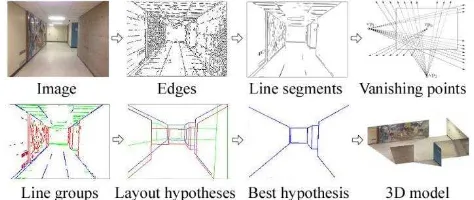
Figure 1. The proposed method detects edges and groups them into line segments. It estimates vanishing points, and creates layout hypotheses. It uses a linear scoring function to score hypotheses, and finally converts the best hypothesis into a 3D model.
In our work, we take the room layout estimation one step further. Our goal is to estimate a layout for a corridor which might be connected to the other corridors from a monocular image. Therefore, there would be no single box constraint for the estimation of the scene layout. We phrase the problem as a hypothesis selection problem which makes use of middle-level perceptual organization that exploits rich information contained in the corridor. We search for the layout hypothesis which can be translated into a physically plausible 3D model. Based on Manhattan rule assumption, we adopt the stochastic approach to sequentially generate many physically valid layout hypotheses from both detected line segments and virtually generated ones. Here, each generated hypothesis will be scored to find the best match. Finally, the best generated hypothesis will be converted to a 3D model. Figure 1, shows the workflow of the proposed method.
The main contribution of the proposed method is the creation of corridor layouts which are no more bounded to the one single box format. The generated corridor layout provides a more realistic solution while dealing with objects or occlusions in the scene. Hence, it is well-suited to describe most corridor spaces, and it outperforms the methods which are restricted to one box primitive for estimating the scene layout. Also, we propose a scoring function which takes advantage of both orientation map and geometric context for scoring the created layout hypotheses. Since no suitable data exists for this task, we also collected our own dataset by taking pictures from York University Campus buildings. We collected images from various buildings, resulting in the total of 78 single images. We labeled our data with rich annotations including the ground-truth layout and the floor plan of each corridor within the buildings. In the following section an overview of the proposed method will be provided.
2. INDOOR CORRIDOR DATASET
The goal here is to estimate indoor corridor layout in a single image. Hence, we collected our dataset by crawling through different indoor locations at York University campus area in Toronto, Canada. We chose different places such as Behavioural Science, Petrie Science, Osgoode Hall and Ross buildings. These buildings were chosen due to their free accessibility over time, presence of indoor corridors which are aligned with Manhattan structure format and also having floor plans. To get the data, we walked through the buildings during weekends and out of many locations, we took some images with sufficient resolution which had clear view of the main and side corridors. Statistic wise, the selected locations in the taken images have in total 297 corridors, 1283 walls, 206 doors, and 53 windows. The number of photos for each corridor ranges from 1 to 5, with the total number in our dataset being 78, not counting the single room images.
We associated the data with different types of ground-truth. We associated the corridor outline, corridor type, as well as the position of doors and windows. Note that we intentionally picked up corridors which have simple and rectangular outline, but not necessarily all the corridors in the dataset do not have a complex polygonal shape. Roughly, less than seven percent of corridors in the dataset have a complex polygonal shape. In each photo we identified the ceiling, floor, front, left, and right wall, for the main corridor as well as the ceiling, floor, right or left wall for the side corridors. In order to identify these planes in an image, the respective corner points of these structural
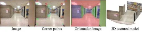
planes were manually pinpointed in the image, and their image coordinates were saved in an individual files. Later on these image coordinates were used to create the ground truth orientation image and 3D model of the corridor layout.
Figure 2. From left to right: sample image from dataset, identified layout corner points, ground truth orientation image and the respective 3D textured model.
It should be noted that in some cases defining the indoor corridor layout in an image is a very challenging task even for a human. This is due to the complex polygonal shape of the building indoor layers. In most cases we resolved the problem by considering the semantics, such as the type of scene, the presence of doors and windows, and sometimes even presence and location of objects. However, there were cases where even humans could not estimate the correct layout. In such cases, we allowed ourselves to omit the ambiguous examples from the dataset. Scene complexity has a governing role in categorizing the created dataset. Scene complexity by itself is a subjective
term which may oppose some confusion to anyone’s mind.
Although various factors have been identified to have an impact on scene complexity, we define scene complexity as a function of three major factors. These factors are: a) scene type or the number of structural planes, b) presence of objects and occlusions, c) length of corridors. Even though explicitly expressing these factors and their impacts on the overall scene complexity was not possible, we implicitly considered these factors for categorization of the prepared dataset. Considering scene complexity, the dataset is partitioned into three image categories which have simple, complex, and very complex indoor layout. Figure 2, shows a sample image from dataset along with identified structural planes corner points, ground truth orientation image and the respective 3D textured model. It should be noted that this dataset will be officially available to the public in the near future.
3. LAYOUT ESTIMATION
While indoor space modeling is possible through applying either top-down or bottom-up approaches, it would be naive to choose any of these approaches without considering their pros and cons. Top-down approaches can be labelled as deterministic, and this labelling could be justified by their dependency on employing strong prior. Hence, top-down approaches are usually more robust to the missing data problem. An example of applying top-down approach is the indoor modeling method presented by Hedau et al. (2009). While top-down approaches are very much deterministic in employing strong priors, bottom-up approaches usually make use of weak priors. Therefore, in bottom-up approaches the perception forms by data. This basically means that if you adopt a bottom-up approach for indoor space modeling, then you expect the created model to be more flexible compare to a model created
by applying a top-down approach (Baligh Jahromi and Sohn, 2015).
Most of the time, indoor modeling using a single image has to deal with the presence of clutters and occlusions in the scene. Hence, missing data problem could be a major issue in using single images for indoor modeling. Since top-down approaches are more robust to the missing data problem, they could be better approaches to be chosen for indoor modeling based on a single image. The proposed method in this paper is more inclined to a top-down approach, and it is governed by this strong prior that the indoor scene layout must have a cubic formation. Yet, what makes this method different from the others is that this method does not restrict the indoor scene layout to be comprised of only one box. The proposed method relaxes the strong prior that indicates the indoor layout is comprised of only one box and let the incoming layout to be comprised of multiple connected boxes. This advantage of the proposed method targets the modeling of occluded areas in the scene.
The overall workflow of the proposed method is as following; 1) Edges are extracted in the single image, and grouped into straight line segments. 2) Line segments will be grouped based on parallelism, orthogonality, and convergence to common vanishing points. 3) Many physically valid major box layout hypotheses will be created using detected line segments and virtual rays of vanishing points. 4) The created major box layout hypotheses will be scored by a linear scoring function. 5) Only 20% of the layout hypotheses which get higher scores will remain in the hypothesis generation pool and the rest will be discarded. 6) The remaining major box layout hypotheses will be deformed by sequentially introducing side box hypotheses to their structure. Note that the maximum number of side box hypotheses which can be integrated to a major box hypothesis is four. 7) The generated side box hypotheses will be also scored, and only the hypothesis which gets the highest score will remain in the hypothesis generation pool. 8) Finally the best fitting layout hypothesis is selected by comparing the scores, and it will be converted to a 3D model.
3.1 Vanishing Points
Single images captured from indoor places are prone to sustain straight line segments. Straight line segments can be detected in an image by linking the extracted edge pixels based on predefined criteria. In most of the manmade structures there are bunch of parallel line segments that converge to the orthogonal vanishing points. Mainly there are four different methods for estimating vanishing points (Bazin et al., 2012): 1) Hough Transform (HT), 2) Random Sample Consensus (RANSAC), 3) Exhaustive Search on some of the unknown entities, and 4) Expectation Maximization.
Here, the Line Segment Detector (LSD) method is applied for extracting straight line segments in an image (Grompone von Gioi et al., 2010). This method is a linear-time line segment detector which can provide sub-pixel accurate results without tuning the parameters. Later, a modified RANSAC approach is applied for estimating vanishing points. In RANSAC approach two straight line segments will be randomly selected and intersected to create a vanishing point hypothesis and then count the number of other lines (inliers) that pass through this point. The drawback of RANSAC is that it does not guarantee the optimality of its solution by considering the maximum intersecting lines as inliers. Here, we follow Lee et al. (2009) to
find three orthogonal vanishing points. In Lee et al. (2009) the coordinates of the RANSAC solution are fine-tuned using non-linear optimization with a cost function.
3.2 Layout Hypotheses Creation
In order to facilitate the indoor modeling using a single image, we forced the indoor scene layout to be comprised of at least five structural planes which simply define a single box. Here, main orthogonal walls in indoor places are at the primary interest to be created compare to windows or doors. Since indoor corridor layouts are not usually bounded to only one box, we define corridor layouts by integration of different single boxes. Hedau et al. (2009) proposed a method for creation of a single box layout hypothesis by sampling pairs of rays from two furthest orthogonal vanishing points on either side of the third vanishing point. However, this approach may not provide acceptable results when dealing with long corridors due to the position uncertainty for the estimated vanishing points. Here, the corridor layout is created by utilization of both detected line segments and sampled rays from vanishing points.
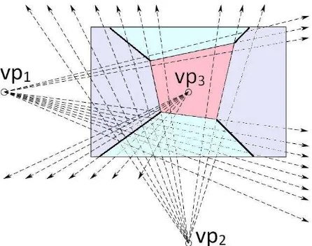
Figure 3. Creating key box Layout hypothesis by intersecting line segments (solid lines) and created virtual rays (dashed lines) using vanishing points.
Here, the corridor layout will be gradually improved from a one box layout to multiple box layouts. Hence, the key box layout hypothesis has to be created first. In order to create the key box hypotheses, let Lx = {lx,1, lx,2, . . . , lx,n} and Tx = {tx,1, tx,2, . . . , tx,n} be the set of actual line segments and virtually generated rays of orientation x, where x Є {1, 2, 3} denotes one of the three orthogonal orientations. A key box layout hypothesis “H” is created by intersecting selected lines from Lx and Tx where the minimum number of selected line segments from Lx is 4, and the total number of all lines needed for this creation is 8. Figure 3, shows the creation of a key box layout hypothesis through intersecting solid and dashed lines which are representing actual line segments and virtually generated rays respectively. Having created the key box layout hypotheses, side box layout hypotheses will be sequentially introduced to every key box layout hypothesis. More detail information on creating layout hypotheses can be found in (Baligh Jahromi and Sohn, 2015).
4. LAYOUT EVALUATION
As mentioned in the previous section, the created layout hypotheses must undergo an evaluation process for selection of the best fitting hypothesis. Here, a linear scoring function is defined to score each hypothesis individually. Given a set of created layout hypotheses in the image space {h1, h2, ...hn} ∈ H, we wish to do the mapping S: H → R which defines a score for every layout hypothesis. The proposed scoring function takes some independent factors into consideration. The proposed scoring function “S” can be decomposed into the sum of three individual scoring functions, which characterize different qualities of the created layout hypotheses. Each of the individual scoring functions is focusing on: a) volume maximization, b) maximization of edge-correspondences, and c) orientation map (OM) and geometric context (GC) compatibility, respectively. These functions, together encode how well the created layout hypothesis represents the scene layout in the image space. We thus have
S(hi) = w1 × Svolume(hi) + w2 × Sedge(hi) + w3 × Som&gc(hi) (1)
where hi = candidate hypothesis S = scoring function
Svolume = scoring function for volume
Sedge = scoring function for edge correspondences Som&gc = scoring function for OM and GC W1,2,3= weight values
It should be noted that the above weight values are define through conducting experimental test on ground truth data. Lee et al. (2010) imposed some volumetric constraints to estimate the room layout. They model the objects as solid cubes which occupy 3D volumes in the free space defined by the room walls. We interpret object containment constraint as the search for the maximum calculated volume among all of the created layout hypotheses. Therefore, a higher score will be given to the layout hypothesis which has a larger volume. In other words, the layout hypothesis which covers a larger area is more probable to contain all of the objects in the room. The calculated score will be normalized to a positive real number between zero and one. The other function which considers edge-correspondences gives the highest score to the layout hypothesis which has the maximum positive edge-correspondences to the detected line segments. This allows the created layout to fit itself as much as possible to the corridor boundaries. The positive edge correspondences is defined by counting the number of edge pixels which are residing close enough to the boundaries of the created layout hypothesis. The compatibility of the created layout hypothesis to the orientation map and geometric context is calculated pixel by pixel. The created layout hypothesis will provide specific orientations to each pixel in the image space, and the orientation map and geometric context are also conducting the same task. Therefore, by comparing layout hypothesis orientation to the orientation provided by the combination of orientation map and geometric context, the better pixel-wise evaluation of the layout hypothesis can be achieved. Since, the combination of orientation map and geometric context is the major contribution of this paper; in the following sub-sections more information in this regard will be presented.
4.1 Orientation Map
Although single images are a reliable data for indoor space modeling, automatic recognition of different structures from a single image is very challenging. Lee et al., (2009) presented the orientation map for evaluation of their generated layout hypotheses. The main concept of the orientation map is to define which regions in an image have the same orientation. An orientation of a region is determined by the direction of the normal of that region. If a region belongs to the XY surface, then its orientation is Z.
Figure 4. Single image, line segments and orientation map. (a) Single image. (b) Detected straight line segments, vanishing point, and two of vanishing lines. (c) Orientation map; regions are colorized according to their orientations.
Orientation map is a map that reveals the local belief of region orientations computed from line segments (Figure 4). If a pixel is supported by two line segments that have different orientations, then this would be a strong indication that the pixel orientation is perpendicular to the orientation of two lines. For instance in Figure 4(b), pixel (1) can be on a horizontal surface because a green line above it and two blue lines to the right and left are supporting pixel (1) to be perpendicular to the orientation of both lines. Also, pixel (2) seems to be on a vertical surface because blue lines above and below and red line to the right are supporting it. Also, there is a green line below pixel (2), but its support is blocked by the blue line between the green line and the pixel. Therefore, the support of a line will extend until it hits a line that has the same orientation as the normal orientation of the surface it is supporting. It means that a line cannot reside on a plane that is actually perpendicular to it.
4.2 Geometric Context
Hoiem et al., (2007) labeled an image of an outdoor scene into coarse geometric classes which is useful for tasks such as navigation, object recognition, and general scene understanding. Usually the camera axis is roughly aligned with the ground plane, enabling them to reconcile material with perspective. They categorized every region in an outdoor image into one of three main classes. First, surfaces which are roughly parallel to the ground and can potentially support another solid surface. Second, solid surfaces those are too steep to support an object. Third, all image regions which are corresponding to the open air and clouds.
Theoretically a region in the image could be generated by a surface of any orientation. To determine which orientation is most probable, Hoiem et al., (2007) used available cues such as material, location, texture gradients, shading, and vanishing points. It should be noted that some of these cues, are only helpful when considered over the appropriate spatial support which could be a region in a segmented image. The common
solution is to build structural knowledge of the image from pixels to superpixels. Hoiem et al., (2007) solution was to compute multiple segmentations based on simple cues. Generally, they sampled a small number of segmentations which were representative of the whole distribution. They computed the segmentations by grouping superpixels into larger continuous segments. Note that different segmentations provide various views of the image. To understand which segmentation is the best, the likelihood that each segment is good or homogeneous must be evaluated. Also, the likelihood of each possible label for each segment must be evaluated. Finally, combination of all the estimates produced by different segmentations would be possible in a probabilistic fashion. Note that a segment could be homogeneous if all of the superpixels inside that segment have the same label. Hoiem et al., (2007) estimated the homogeneity likelihood using all of the cues and boosted decision trees.
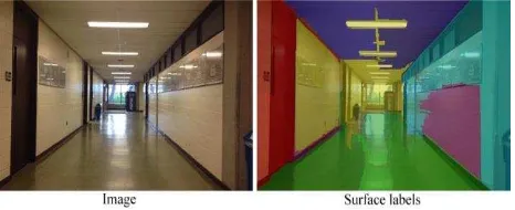
Figure 5. Single image, and the estimated surface labels.
Hedau et al., (2009) used the same idea for labeling surfaces in an image, but this time the main focus was on indoor places and recovering the spatial layout of cluttered rooms. They tried to achieve an overall estimate of where the objects are, in order to get a more accurate estimate of the room layout. To estimate the room layout surface labels including the objects, they use a modified version of Hoiem et al., (2007) surface layout algorithm. The image is over-segmented into superpixels, and in the next step partitioned into multiple segmentations. Color, texture, edge, and vanishing points are the main cues which were computed over each segment. A classifier (boosted decision tree) is used to estimate the likelihood that each segment contains only one type of label and the likelihood of each of possible labels. Further, over the segmentations these likelihoods would be integrated to provide label confidences for each superpixel. Figure 5, Shows an image with its estimated surface labels.
4.3 Orientation Map and Geometric Context Combination Zhang et al., (2014) applied both orientation map and geometric context on overlapping perspective images. In their paper, they expressed that the geometric context can provide better surface normal estimation at the bottom of an image, while the orientation map works better at the top of an image. Hence, they combined the top part of the orientation map image and the bottom part of geometric context image, and used the incoming result to evaluate the room layout. This drastic variation in the performance of orientation map and geometric context from the top to the bottom of the images is explainable. Since most of the images in their dataset were captured from single rooms, either this variation is due to the presence of clutters in most rooms, or because their model was trained based on images looking slightly downwards.
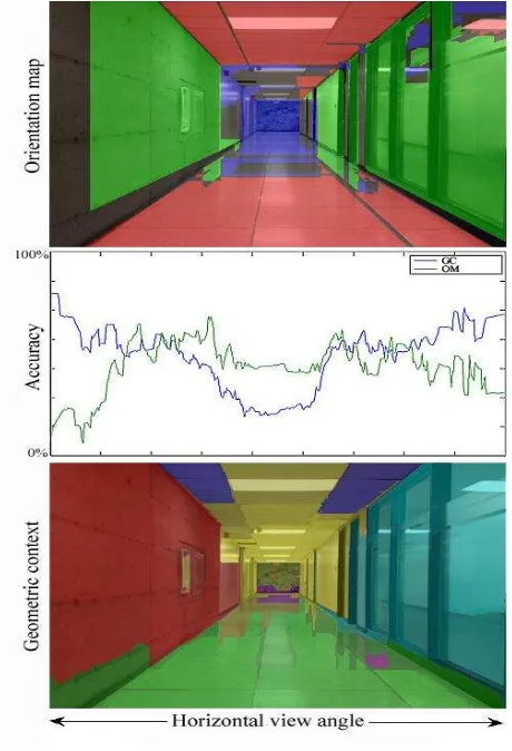
Unlike single rooms which are usually small in size and full of clutters, corridors are usually less occupied with clutters and have longer length. Therefore, we examined the horizontal view angle in the image to evaluate the performance of orientation map and geometric context in the corridor related images. Figure 6, shows the changes in the accuracy of orientation map and geometric context compare to the ground truth training images. As it can be seen in this figure, by changing the horizontal view angle from left to the right side of the image, the orientation map and geometric context performances are varying to a considerable extent. The geometric context is outperforming the orientation map around both sides of the images, while the orientation map is outperforming the geometric context around the center of the images. Here, the combination of orientation map and geometric context is performed by considering their respective performance curves with respect to the horizontal view angle. The combination of these two looks to be a very simple task, yet orientation map and geometric context have little differences in their representation. Hence, their representation must be standardized before the combination would be possible.
Figure 6. Orientation Map and Geometric Context accuracy changes by changing the horizontal viewing angle.
On one hand, the orientation map is not numerically expressed, and on the other hand the geometric context is expressing the likelihood of each possible label for all superpixels in the image. As mentioned before, the orientation map is a map that reveals the local belief of region orientations in an image. These
local orientations are assigned to the image regions through examining their supporting line segments. Usually the orientation map is colorized with four different colors which are red, green, blue, and black. The first three colors are representing a specific orientation in 3D space which is either X, Y, or Z. Normally the black color represents the unsupported regions in an image. Since there is a possibility that some regions in a specific image could not get complete support from line segments, those specific regions would be colorized as black and officially would not be assigned with any orientation.
As mentioned earlier, a specific orientation can be assigned to a local region in an image. Moreover, the assigned orientation can be expressed numerically. In other words, it is possible to say how good the assigned orientation is. To express the orientation map numerically for every region in an image, the supporting line segments should be in focus. Here, image regions will get a value between zero and one for their assigned orientation by considering the length of their supporting line segments. In other words, when a region is fully supported by the longest detected line segments in an image, it will get a value of one for its assigned orientation. Also, when a region is supported by the smallest detected line segments in an image, it will get the value of zero for its assigned orientation. Following the same rational, all the regions in the orientation map image will get a value between zero and one for their assigned orientation. It should be noted that in single images a small line segment might be longer than what it looks in real world due to the perspective effect. Therefore, we used the vanishing points and project all the detected line segments to the image borders to suitably compare their lengths.
After providing different values to the regions orientation in the orientation map image, we had to express the surface labels of geometric context as orientations. Hence, the geometric context has been expressed by the three different orientations which are suggested by the orientation map. Finally, it was possible to combine the incoming results of the orientation map and geometric context with respect to the horizontal view angle in the image. Formulas below are showing how these values can be used for evaluating an individual layout hypothesis:
kx,y = ,
, + , (2) px,y = kx,y× OMx,y
qx,y = (1 – kx,y)× GCx,y
Ix,y (OM, GC) = max (px,y , qx,y )
Som&gc (hi) = 1- ×1 × ∑=1∑ =1(| , (��,��) − , ℎ� |)
where axy = accuracy of OM at pixel (x,y) bxy = accuracy of GC at pixel (x,y) hi = candidate hypothesis
Jx,y (hi) = hypothesis hi orientation value at pixel (x,y)
Ix,y(OM, GC) = OM and GC integration at pixel (x,y) OMxy= orientation map outcome at pixel (x,y) GCxy = geometric context outcome at pixel (x,y) Som&gc (hi) = scoring function for OM and GC
5. EXPERIMENTS
As mentioned in the dataset section, ground truth orientation images were provided for York University dataset. The provided dataset is divided into two categories of training set and testing set. Out of 78 images in the dataset, 53 images were chosen for testing and the rest of 25 images were chosen for training. The training set is used for identifying the accuracy curves related to the horizontal viewing angle changes through both orientation map and geometric context. Since, the ground truth orientation images were provided for each image in the dataset, the comparison between the estimated layout for each test image and the ground truth layout is accomplished. For each test image a quantitative table was produced for better examining the incoming results. The incoming tables were used for evaluating the overall performance of the generated corridor layouts. The average percentage of pixels that have the correct orientation for each image in the test set is 71%. Also, 79% of the images had less than 20% misclassified pixels. However, only 18% of the images had less than 5% misclassified pixels.
Figure 7. Scale ratios between the 3D reconstructed ground truth layouts and the created layouts for 27 images.
Not only the orientation difference in 2D space of the image is a measure for evaluating the estimated corridor layouts, but also the 3D reconstructed layout could be considered for evaluation. Here, 3D reconstruction of the layouts is performed following the proposed approach in Lee et al. (2009). Hence, three
different parameters (λx, λy, λz) are defined for the layout key
box in the object space. λx defines the ration between the width
of the 3D reconstructed layout, and the width of the ground
truth layout. Same as λx, λy and λz compare the length and
height of the 3D reconstructed layout to the length and height of the ground truth layout. Figure 7, shows the scale ratios between the reconstructed layouts key box and their ground truth layouts for 27 images. These images have almost the same scene complexity, so that the comparison of their reconstructed layouts is possible. As it can be seen in Figure 7, the proposed method was more successful in the estimation of scene layout
width and height (λxand λz are close to 1) over the images.
However, it has more problems in estimation of the true length
of the corridors (λy is to some extent not close to 1). This is a
very critical issue and it has to be scrutinized carefully in the future.
In some images, the floor-wall boundary was partially occluded by the objects or human bodies. However, the proposed method could successfully recover the corridor layout in many images. The proposed method makes use of both detected line segments and virtually generated ones to create layout hypotheses. However, our experiment shows that virtual rays cannot be always helpful, especially when the corridor length is very large. In these cases the estimated vanishing points might not
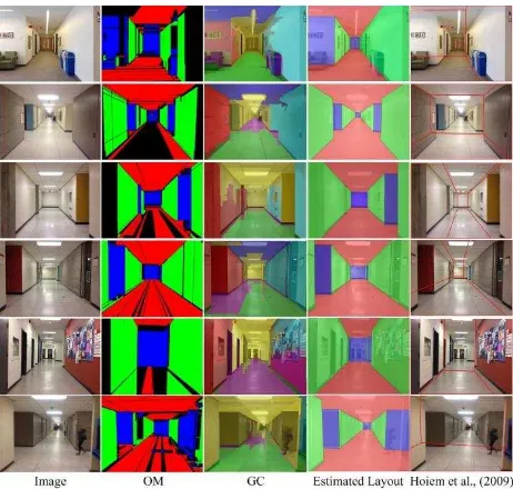
have sufficient position accuracy. Therefore, the created virtual rays will be deviated from the actual layout borders as the ray gets closer and closer to the camera. Although the overall performance of the proposed method is promising, there are some failure cases too. These failures are mostly because of inability to identify orthogonal vanishing points in the image, detection of wrong line segments on glass surfaces or waxed floors, misaligned boundaries, no lines supporting down the corridor or fully occluded floor-wall boundaries. Some of the successful and failure cases of the proposed method in creation of corridor layouts are shown in Figure 8. Considering Figure 8, some of the created layout hypotheses are deviated from the ground truth. The most conspicuous problems are: a) wrong depth estimation for the key box hypothesis, b) wrong side box estimation. Although the algorithm could manage to select the correct number of boxes in most of the images, it could not filter out inaccurate edges (edges detected on the glass surfaces).
Figure 8. Examples of both successful and unsuccessful estimations for indoor corridor layouts are above.
6. CONCLUSION
The main focus of this paper is on 3D modeling of indoor corridors using a single image. 3D modeling of indoor spaces is not a trivial task, and it involves with major problems. These problems may directly inherit from the modeling approach itself, or the adopted data gathering technique. In this paper, the proposed indoor corridor layout estimation approach is following the Manhattan rule assumption to simplify the structure of the indoor corridor layouts. What does make the proposed method more conspicuous than the other methods is that the incoming estimated layout is not restricted to only 1 box. We addressed the indoor corridor layout estimation problem by hypothesizing-verifying multiple box primitives. The proposed method applies the middle-level perceptual organization. It relies on both detected line segments and virtual rays created by orthogonal vanishing points to estimate indoor corridor layouts. The proposed method can easily handle the presence of accessory hall ways and occlusions in corridor
scenes even the objects were occluding some parts of the floor-wall or ceiling-floor-wall boundaries. This feature beside the compatibility of the estimated layout to the combination of orientation map and geometric context are the main advantages of the proposed method. The proposed method shows by applying a prior knowledge, the 3D layout of an indoor scene can be successfully recovered using a single image. A very interesting future problem would be the integration of individual indoor layouts which is a huge step towards complete indoor space modeling.
ACKNOWLEDGEMENTS
This research was supported by the Ontario government through Ontario Trillium Scholarship, NSERC Discovery, and York University. In addition, the authors wish to extend gratitude to Miss Mozhdeh Shahbazi, who consulted on this research.
REFERENCES
Baligh Jahromi, A. and Sohn, G., 2015. Edge Based 3D Indoor Corridor Modeling Using a Single Image. ISPRS Annals of the Photogrammetry, Remote Sensing and Spatial Information Sciences, Volume II-3/W5, pp. 417–424.
Bazin, J.C., Seo, Y., Demonceaux, C., Vasseur, P., Ikeuchi, K., Kweon, I. and Pollefeys, M., 2012. Globally Optimal Line Clustering and Vanishing Point Estimation in Manhattan World. In: Proceedings of 25th IEEE Conference in Computer Vision and Pattern Recognition, pp. 638-645.
Chao, Y.W., Choi, W., Pantofaru, C., and Savarese, S., 2013. Layout estimation of highly cluttered indoor scenes using geometric and semantic cues. In: Proceedings of the International Conference on Image Analysis and Processing, pp. 489-499.
Fidler, S., Dickinson, S., and Urtasun, R., 2012. 3D object detection and viewpoint estimation with a deformable 3D cuboid model. In: Advances in Neural Information Processing Systems, pp. 611–619.
Gioi, R. G., Jakubowicz, J., Morel, J. M., Randall, G., 2010. LSD: A Fast Line Segment Detector with a False Detection Control. IEEE Transactions on Pattern Analysis and Machine Intelligence, vol. 32, no. 4, pp. 722-732.
Han, F., and Zhu, S.C., 2005. Bottom-up/top-down image parsing by attribute graph grammar. In: Proceedings of the IEEE International Conference on Computer Vision, vol. 2, pp. 1778–1785.
Hedau, V., Hoiem, D., and Forsyth, D., 2009. Recovering the spatial layout of cluttered rooms. In: Proceedings of the 12th IEEE International Conference on Computer Vision, pp. 1849– 1856.
Hedau, V., and Hoiem, D., 2010. Thinking inside the box: using appearance models and context based on room geometry. In: Proceedings of the European Conference on Computer Vision, pp. 1–14.
Hedau, V., Hoiem, D., and Forsyth, D., 2012. Recovering free space of indoor scenes from a single image. In: Proceedings of the IEEE Conference on Computer Vision and Pattern Recognition, pp. 2807-2814.
Hoiem, D., Efros, A., and Hebert, M., 2005. Geometric context from a single image. In: Proceedings of the IEEE International Conference on Computer Vision, pp. 654–661.
Hoiem, D., Efros, A. A., & Hebert, M., 2007. Recovering surface layout from an image. International Journal of Computer Vision, vol. 75, no. 1, pp. 151–172.
Kosecka, J., and Zhang, W., 2005. Extraction, matching, and pose recovery based on dominant rectangular structures. Computer Vision and Image Understanding, vol. 100, pp. 274– 293.
Lee, D.C., Hebert, M., Kanade, T., 2009. Geometric reasoning for single image structure recovery. In: Proceedings of the IEEE Conference on Computer Vision and Pattern Recognition, pp. 2136–2143.
Lee, D.C., Gupta, A., Hebert, M., Kanade, T., 2010. Estimating spatial layout of rooms using volumetric reasoning about objects and surfaces. In: Advances in Neural Information Processing Systems, pp. 1288-1296.
Liu, C., Schwing, A.G., Kundu, K., Urtasun, R. and Fidler, S., 2015. Rent3D: Floor-plan priors for monocular layout estimation. In: Computer Vision and Pattern Recognition (CVPR), pp. 3413-3421.
Micusik, B., Wildenauer, H., Kosecka, J., 2008. Detection and matching of rectilinear structures. In: Proceedings of the IEEE Conference on Computer Vision and Pattern Recognition, pp. 1-7.
Pero, L., Bowdish, J., Fried, D., Kermgard, B., Hartley, E., and Barnard, K., 2012. Bayesian geometric modeling of indoor scenes. In: Proceedings of the IEEE Conference on Computer Vision and Pattern Recognition, pp. 2719-2726.
Schwing, A. G., Hazan, T., Pollefeys, M., Urtasun, R., 2012. Efficient Structured Prediction for 3D Indoor Scene Understanding. In: Proceedings of the IEEE Conference on Computer Vision and Pattern Recognition, pp. 2815-2822.
Schwing, A. G., Urtasun, R., 2012. Efficient Exact Inference for 3D Indoor Scene Understanding. In: Proceedings of the European Conference on Computer Vision, pp. 299-313.
Schwing, A. G., Fidler, S., Pollefeys, M., Urtasun, R., 2013. Box in the box: Joint 3d layout and object reasoning from single images. In: Proceedings of the IEEE International Conference on Computer Vision, pp. 353-360.
U.S. Environmental Protection Agency, 2015. The inside story:
a guide to indoor air quality.
http://www.fusionsvc.com/The_Inside_Story.pdf (accessed July 2015).
Wang, H., Gould, S., Koller, D., 2010. Discriminative learning with latent variables for cluttered indoor scene understanding. In: Proceedings of the European Conference on Computer Vision, pp. 435-449.
Yu, S., Zhang, H., Malik, J., 2008. Inferring spatial layout from a single image via depth-ordered grouping. In: Proceedings of the IEEE Workshop on Perceptual Organization in Computer Vision, pp. 1-7.
Zhang, Y., Song, S., Tan, P., & Xiao, J., 2014. PanoContext: A whole-room 3D context model for panoramic scene understanding. In: Proceedings of the European Conference on Computer Vision, pp. 668-686.