LOCALIZATION OF WINDOWS AND DOORS IN 3D POINT CLOUDS OF FACADES
William Nguatem, Martin Drauschke, Helmut Mayer
Institute of Applied Computer Science Bundeswehr University Munich
Werner-Heisenberg-Weg 39, 85577 Neubiberg, Germany william.nguatem,martin.drauschke,[email protected]
http://www.unibw.de/inf4/professuren/photo/index_html
Commission III/2,4
KEY WORDS:Point Cloud, Object Localization, Splines, Model Selection, Non-linear Regression Fitting, Markov Chain Monte-Carlo
ABSTRACT:
In this paper, we present a fully automatic approach to localize the outlines of facade objects (windows and doors) in 3D point clouds of facades. We introduce an approach to search for the main facade wall and locate the facade objects within a probabilistic framework. Our search routine is based on Monte Carlo Simulation (MC-Simulation). Templates containing control points of curves are used to approximate the possible shapes of windows and doors. These are interpolated using parametric B-spline curves. These templates are scored in a sliding window style over the entire facade using a likelihood function in a probabilistic matching procedure. This produces many competing results for which a two layered model selection based on Bayes factor is applied. A major thrust in our work is the introduction of a 2D shape-space of similar shapes under affine transform in this architectural scene. This transforms the initial parametric B-splines curves representing the outlines of objects to curves of affine similarity in a strongly reduced dimensionality thus facilitating the generation of competing hypotheses within the search space. A further computational speedup is achieved through the clustering of the search space to disjoint regions, thus enabling a parallel implementation. We obtain state-of-the results on self-acquired data sets. The robustness of our algorithm is evaluated on 3D point clouds from image matching and LiDAR data of diverse quality.
1 INTRODUCTION
The modeling of architectural scenes is a very busy research topic and can be viewed from very different perspectives: The nature of the data (images vs. LiDAR, aerial vs. terrestrial), its scale (building vs. city), or its purpose, e.g., cultural heritage, construc-tion planning or touristic applicaconstruc-tions. Consequently, the em-ployed methodologies also differ. For examples, Lin et al. (2013) concentrate on fast data processing methods to reconstruct subur-ban areas from a mobile mapping system using LiDAR, Lafarge and Mallet (2012) derive a scene representation at city-scale in which simple surfaces are modeled by geometric primitives, and complex structures are represented by a triangular mesh. While Friedman and Stamos (2013) focus on repetitive structures of modern buildings, Brandenburger et al. (2013) extract ornamental details from images of historical facades.
Since man-made objects like buildings show a rich diversity in size, shape, or style, all approaches for reconstructing, approxi-mating or interpreting such data have to deal with model selec-tion, i.e., methods for fitting and comparing competing models to the acquired data are employed. If scenes are only coarsely mod-eled, the presentation of the approaches often concentrate on data representation, e.g., (Lafarge and Mallet, 2012), or the focus of the publication lies on the modeling of domain knowledge or its transfer during the data analysis, e.g., (Becker and Haala, 2008; Friedman and Stamos, 2013; Lin et al., 2013). The model selec-tion is often only sketched. In contrast, when modeling smaller structures, often several models roughly fit to the data. Then in this case model selection methods are often discussed to demon-strate the plausibility of the model refinements, e.g., (Alegre and Dellaert, 2004; Dick et al., 2004; Brandenburger et al., 2013).
Which model fits best to the data? This is a very old and philo-sophical question. Already in the 14th century, William of
Ock-ham stated that it is better to choose a simple model than a com-plex one. This principle is known as Occam’s razor. Since this judgement is sensible, many modern model selection approaches in computer sciences consider both, the closeness of the model to the data, and the model complexity. E.g., Akaike (1973) de-rived his selection criterion from information theory, and Ris-sanen (1987) proposed the minimum description length (MDL) principle for choosing the best model, i.e., he evaluates its size for representation.
A probabilistic view on model selection is proposed by Ale-gre and Dellaert (2004) who interpret a rectified facade im-age by its stepwise division in meaningful parts of rectangular shape. The segmented parts are interpreted by a Bayesian gener-ative model which was constructed from a context-free grammar. Markov Chain Monte Carlo (MCMC) sampling is employed to derive posterior probabilities for each part. Another probabilistic Bayesian framework is proposed by Dick et al. (2004) who use one complex model for windows of several shapes, e.g., with arch height and bevels on the one hand, and various priors, e.g., on ob-ject shape and position on the other hand. The evaluation is based on likelihoods derived from image intensities of backprojected fa-cade objects. Besides the high complexity of the MCMC-based search for facade objects, the approach has another deficit regard-ing the assumption on normalized illumination condition and a uniform material characteristic of each object. In probabilistic approaches, model complexity is considered when defining like-lihood terms, e.g., (Dick et al., 2004), or in the probabilities for jumps of the reversible jump Markov Chain Monte Carlo (rjM-CMC) framework, e.g., (Ripperda and Brenner, 2006).
edge points in the point cloud, and an axis-aligned cell decom-position to obtain outlines of doors and windows. The authors state that arch-shaped doors can also be considered, but the cor-responding model selection step is not discussed in (Becker and Haala, 2008). We assume that the classification is performed by a decision stump, hence arches with a small height are not de-tected. Recently, Fritsch et al. (2013) adopted the approach to dense point clouds derived from 3D reconstruction. Another ap-proach for building analysis in LiDAR point clouds is presented by Schmittwilken et al. (2009) who derive the scene interpretation by employing a conditional random field and an attribute gram-mar to interpret geometrical entities which were recognized be-fore. While this approach combines a probabilistic and a flexible model-based interpretation, the shape of the recognized building parts only relies on the previous segmentation step which is some-how similar to (Becker and Haala, 2008). As third example, Tut-tas and Stilla (2013) derive building models from oblique ALS, and they derive window hypotheses from 3D points reflected by objects within the rooms (voyeur effect) assuming glass windows. Only rectangular shaped windows are presented in their results, although the facade shows arch-shaped windows.
All the mentioned state of the art approaches have one step in common: First a coarse building model is determined, i.e., the major planes of ground, facade and roof, and then, it is refined in a successive step. Yet, in our experiments we saw that it is some-times difficult or even impossible to find the perfect facade plane, because of a highly structured facade in 3D due to ornaments, balconies and oriels, or because of the building construction, es-pecially considering historical buildings and old buildings in rural areas. Consequently, state of the art approaches may have prob-lems when detecting building parts in such environments. We want to overcome this drawback by considering a discrete set of segmented planes for facade hypothesis rather than a single per-fect segmentation of the facade.
In this paper we propose a window and door detection based on sampling with only few iterations, which works well on various kinds of facades with a geometric structure in 3D, and as demon-strated in our experiments we are able to reliably distinguish be-tween various window and door shapes. Specifically, we want to estimate a precise outline of all windows of a facade, which has been reconstructed from image sets by recent approaches, e.g., (Snavely et al., 2006; Frahm et al., 2010; Mayer et al., 2012). We use MC-Simulation to generate and score competing mod-els and apply a model selection based on Bayes factor. For the parametrization of the models, we use the notion of sub-space from (Isard and Blake, 1998) which originally has been proposed in the field of object contour tracking.
The rest of the paper is structured as follows; In Section 2, be-ginning with an introduction, we present our probabilistic facade object localization algorithm in its entirety. This is followed by a thorough discussion of our results in the evaluation presented in Section 3, and finally, in Section 4, we conclude and present possible future work.
2 PROBABILISTIC OBJECT LOCALIZATION ON FACADES
2.1 Overview of the Algorithm
The input to our system is an unstructured 3D point cloud,D, containing one or more building facades. This could have origi-nated from image matching or LiDAR. The output are fitted con-tours defining the outlines of windows and doors. We divide the
work flow of our algorithms into three main stages: Facade Seg-mentation, Window and Door Localization, and Model Selection. Within the Facade Segmentation, assuming that Dunderlies a known metric scale and the gravity (up) vectorvis known, we extract facades planes and estimate the outlines of interesting ob-jects present on the facade. In the localization stage, making no assumptions about the occurrences of windows and doors on fa-cades, we build probability distributions of these objects on every location of the facade by matching predefined templates on the estimated outlines. This results in multiple detections of compet-ing templates. We remedy this durcompet-ing the model selection stage. Figure 1 depicts the detailed work flow of our algorithm.
2.2 Facade Segmentation
There exist a plethora of work describing oriented plane segmen-tation in 3D point clouds. However, in the real world, a single segmented vertical plane from the 3D point clouds of a facade is hardly enough to capture information about the true boundaries of facade objects e.g. windows. Reasons are for instance architec-tural imperfections, variability in shapes and styles of windows and doors as well as variability in the distances these off-the-facade objects protrude from the true off-the-facade. Also, a possible unequal point distribution on the facade originating from textural differences could possibly be an additional problem. To remedy this we first segment a single vertical plane using MSAC from (Torr and Zisserman, 2000). This serves as a starting hypothe-sis for the construction of a discrete probability distribution over facades. We sweep this first segmented plane along its normal direction, whilst randomly changing the angle of the vertical di-rection (the value ofv) at each sweeping step. We call this pro-cedure a plane-angular sweep. The small and random changes in vduring plane sweeping ensures the construction of an ensem-ble of planes slightly but non-parallel to the first main segmented plane. For the plane-angular sweeping, a finer inlier threshold is used compared to that used within MSAC to segment the first plane. ForMsuch plane-angular sweeps, the output for a given facade are a finite set ofMsegmented planes,{F(i)}M
i=1, used
as a discrete representation ofp(F|D), the probability of the true facade given the data. For each element of{F(i)}M
i=1, we
esti-mate boundary points using a boundary estimation algorithm e.g. (Rusu et al., 2007). These boundary points{B(i)}M
i=1, are a
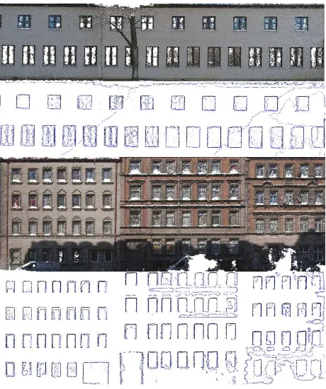
dis-crete approximation of the probability of the outlines of facade objects. Figure 2 shows on the left side the inliers of two plane-angular sweeps of a reconstructed facade points and the right side depicts hypothesis of the estimated object boundaries. Taking the windows on this facade as an example, a single facade hypothe-sis from plane segmentation makes only a partial coverage of the presence and locations of these facade objects. In some simple cases, a single sweep’s boundary hypothesis can reveal almost all the outlines of windows and doors. This is the case shown in 3 for these facades gained from 3D point clouds from image matching.
Optionally, for buildings whose windows and doors protrude very little from the facade, surface curvature of 3D points are esti-mated using e.g. algorithms presented in (Nguatem et al., 2012). Points exhibiting high curvature values are then fused to every element of{B(i)}M
i=1.
2.3 Window and Door Localization
The goal of the detection stage is to localize portions of{B(i)}M
i=1
with high probability of being the outlines of windows and doors. Using orthogonal projection, we convert these boundary esti-mates from 3D to 2D points,{B(i)2D}M
i=1. On every element of
{B(i)2D}M
Figure 1:Block diagram of the complete algorithmic work flow. An optional clustering is used to divide the search space to enable a parallel implementation. Also the fusion of surface curvature values is optional and only needed for facades whereby, windows and doors are only slightly off the main facade plane thus providing little 3D geometrical information. This can be found particularly in some modern buildings.
Figure 2:The left side shows two hypothesis from plane-angular sweep segmentation of the same facade and the corresponding outlines are shown on the right. These combined outlines in most cases reveals the correct outlines of windows and doors.
search and score predefined templates for windows and doors us-ing a window and door likelihood function. In Figure 3, we can see that huge portions of the boundary estimates contain no 3D point. Optionally, to avoid sliding over these big empty regions, we cluster{B2D(i)}M
i=1and apply the sliding window only on
clus-ters of reasonable sizes. For very long facades, this results in a significant speedup.
2.3.1 Notation, Model Definition and Parametrisation Be-fore explaining our probabilistic template matching algorithm, we first define the notations used and the choice of parametri-sation for window and door templates. Figure 4 illustrates the span of windows and door models used during this research and the corresponding templates. Analogous to approaches on shape analysis, e.g., Ferrari et al. (2006) and Riemenschneider et al. (2010), we define these templates by control points (the blue stared markers) whose 2D coordinates when interpolated gives the full outlines (the red curves) of the model r(s). This in-terpolation is performed using parametric B-spline curves and is defined as follows
r(s) =
B(s)T 0
0 B(s)T
Q (1)
whereQ = (x1, x2, x3, . . . , xN, y1, y2, y3, . . . , yN)T defines
the coordinates of the control points,B(s)a spline basis function andN is the number of control points. The choice of
interpola-Figure 3: The point clouds of two facades are shown above a single hypothesis boundary estimates. The boundary estimates reveals the outlines of most windows and doors present on the facades.
tion using the B-spline representation brings along some advan-tages: First, this representation enforces the natural smoothness inherent in the object outlines. Secondly, this turns out to be more robust to measurement noise than explicit parametrisation, and it reduces the dimensionality considerably. We further reduce the dimensionality of these templates by defining a mapping from the spline space of control points to a much lower dimensional sub-space, the 2D affine shape-space, with a shape-space vector,
θ, given by
Q=Wθ+Q0 (2)
whereQ0defines the template, andWthe shape-space matrix.
Wis defined as
W=
1 0 Qx0 0
0 1 0 Qy0
Figure 4: The span of windows and doors templates,Q0, used
during this work. This ranges from the simple rectangular rep-resented by the four corner points (marked blue) through the arched-dormer, half-circular and gothic windows and doors rep-resented by many more control points.
where0= (0,0, . . . ,0)Tand1= (1,1, . . . ,1)T. Qx 0andQ
y 0
are the decomposition of the template curveQ0into vectors of
itsxandycoordinates respectfully. Thus mapping in equation (2) can be written as follows
Elements ofθare given by
θ= (tx, ty, sx, sy)T,where
tx=a shift in the x-axis ty=a shift in the y-axis
sx=scaling in the x-axis sy=scaling in the y-axis
Examples of 2D shape-space vectors and the respective meaning of the affine transformations on the template are:
• θ= (0,0,0,0)T
,the original templateQ0
• θ= (0,1,0,0)T
,Q0shifted 1 unit to the left
• θ= (0,0,1,1)T
,Q0doubled in size.
This mapping ensures that changes in the components ofθresults in all the necessary affine transformations of similarities by our templates. We neglect a rotation term since windows and doors are assumed to be placed up-right on the facade, knowing that our vertical up direction is reliable. Ifθis defined over a com-pact supportS, then for a given template from the span, the only elements ofθwhich are expected to vary aresxandsyto
en-able the capturing of the different windows and door sizes andtx
andtyfor shifting the templates to different positions of the
fa-cade. However, the later is implicitly gained through the sliding of the template over the facade and is deterministic. This leaves an effective dimensionality of two and therefore substantiates the choice of shape-space over the spline space parametrisation.
2.3.2 Template Likelihood Computation In this section we derive a measure of how good a realization ofθfromSexplains the data. Ideally, we would like a template, when placed on a particular position on an element of{B(i)2D}M
i=1to exhibit perfect
fit, i.e. all the inliers should lie uniformly spread on the interpo-lated curve. MSAC is usually used to capture the goodness of the fit. A good approximation of the point spread is the standard deviationσ(θ) of the number of inliers along the curve. This value is inversely proportional to the goodness of the inliers point spread. Uniformly spread inliers have a lower standard deviation than non-uniformly spread points. These two terms, normalized between 0 and 1 are combined to define our window or door out-line likelihood function as follows
L(θˆ)∝w(θ) +σ(θ), (5)
Figure 5:The bottom row shows on the left hand side the input 3D point clouds and the right hand a single element of{B2D(i)}M
i=1. An
enlarged portion of the red marked area is shown on the top row. The green crosses are the boundary points, the brown pluses are 100 interpolation points of the B-spline curve used in fitting the data. The inliers of these curves are shown by the yellow crosses.
where
e2k is the shortest distance from the 2D pointpkto the
interpo-lated template curve defined byθandT is the inlier threshold. The summation indexk runs over all the points in the element of{B2D(i)}M
i=1considered. In Figure 5, the green crosses are the
boundary points and the brown pluses represents 100 points on the interpolated curve for the template of a half-circular window. It may seem that the interpolated curve on the left side of the top row of the Figure has a better fit to the data than the one on the right side (the yellow crosses represent the inliers). Yet, the in-liers on the curve of the right hand side show a better average spread (lowerσ(θ)) than the ones on the right. This results in
an overall reduction in the likelihood of the curve on the right to that on the left and substantiates our choice of likelihood function over the vanilla MSAC.
2.3.3 Probabilistic Template Matching We define the goal of the probabilistic template matching as follows: Given a com-pact supportSoverθ, and a span of templates, compute the like-lihood (L(θ)1,L(θ)2,L(θ)3, . . .L(θ)N) ofNrealisations ofθ for every position of each element of{B(i)2D}
M
i=1and find the
max-imum. We defined this optimization as follows
ˆ
θ= argmax θ∈S
(L(θ)) (8)
For each templateQ0from the span, we solve this optimization
using MC-Simulation in the algorithm depicted in Algorithm (1).
Data:{B2D(i)}M
i=1,Q0
Result:θˆ1,θˆ2, . . .
initialization; whilei <Mdo
whilej <N do
θ∼S (i.e. sample θ uniformly from S) Get the control points,Q, using equation (2) InterpolateQto getr(s)using equation (1) Scorer(s)onB(i)2Dusing equation (6) end
Getθˆwith highest score using equation (5) end
Algorithm 1:Probabilistic template matching.
Categories Type-1 Type-2 Type-3
hdoor 0.8m - 1.3m 1.7m - 2.3m 1.3m - 1.7m
wdoor 0.8m - 1.4m 1.4m - 2.3m 2.3m - 3.0m
hwindow 1.8m - 2.6m 2.6m - 3.3m 3.3m - 3.5m
wwindow 0.8m - 1.4m 1.4m - 2.0m 2.0m - 3.5m
Table 1:Variations of window and door heights and widths of our experiments. These define a compact supportSoverθ.
and doors heights (hd) and widths (wd) respectively and this
intend defines the compact supportSoverθ.
A snapshot of the results of this probabilistic template matching for the input data from Figure 5 is shown in Figure 6 for two different templates. This reveals the problem of multiple detections. Our approach to solving this problem is presented in the next section.
2.4 Model Selection
For the rectangular template, linear parametric B-spline curves (also known as a spline of degree one) are used for interpolation. This is equivalent to connecting the four corner points of the rect-angle shown in Figure 4. For the other templates, quadratic B-spline curves (B-splines of degree two) are employed to produce smooth interpolated curves. Though most popular model selec-tion approaches, e.g. AIC, explicitly need to include this differ-ence in dimensionality, we argue that the Bayes factor implicitly penalizes complex models compared to simpler ones when sam-ples are generated from independent and identically distributed (i.i.d) random variables.
The problem of multiple detections can be divided into two main groups: Overlap detection of different templates and overlap de-tections of the same template but sampled from different cate-gories of the compact support. In a model selection sense, these are all competing detections. We apply a two layered solution called inter class model selection and intra class model selection, respectively.
2.4.1 Intra Class Model Selection Here, all models originate from one and the same template from the span and the ultimate goal is to select one of the category (Type-1, Type-2, Type-3) from Table 1. Let us consider the case where we are using a rect-angular template. Using only two samples, i.e.,N = 2, for each category of the compact support, Figure 7 shows screen shots of the output for a given run of our algorithm at a given position while sliding over an element of{B2D(i)}M
i=1. The yellow points
represent the inliers and the corresponding sampled rectangular curve (brown pluses) depicts a window hypothesis. It can be seen that the two rectangles on the lower row fit this data better than
Figure 6:Multiple detections of a half-circular and a gothic win-dow models.
Figure 7:Intra class model selection using the simple rectangular template. The upper row depicts two samples (the brown pluses) of a rectangular template of Type-2 from Table 1 while the lower row shows two samples of Type-1. The strong evidence of Type-1 rectangular window over Type-2 can be seen by the higher num-ber of inliers (yellow crosses) on the samples of the lower row.
the two on the upper row. Since the likelihood function captures the goodness of this fit, one of these two lower rectangles would have the highest score forL(θ). We call this the maximum a posteriori sample (MAP),θrectfor the rectangular template. In
accordance to Bayes factor, we select the category from where
θrectwas sampled (Type-1) in this case.
2.4.2 Inter Class Model Selection Having solved the prob-lem of intra class model selection on all sliding positions as ex-plained above, over the entire facade MAP values are available for all templates from the span, i.e.θgothic,θarc,θcircle. Now, the ultimate goal is to choose one of the four competing tem-plates. Again, in accordance with Bayes factor, at a given posi-tion on the facade we chose the template whose MAP value at that position is highest. Finally, we select all non-overlapping curves with the highest MAP values. Example MAP estimates of an arched-dormer and a gothic window are compared in Figure 8 demonstrating our inter class model selection.
Figure 9: The diagram shows localization results of two different facades. The outlines filled in red giving 3D polygons represent windows and doors. The dimensions of window and door estimates may not be the same. This is because these estimates are from i.i.d random variables. This can be seen on three of the doors on the right facade.
Figure 12:Filled red polygons representing localized windows and doors. Most often, segments of these outlines are embedded within the 3D point clouds of the facade. As mentioned in Figure 9, dimensions of windows and doors estimates may not be the same.
Figure 8: Inter class model selection between templates of a gothic (brown pluses on the left side) and an arched-dormer (right side) window. The inliers (yellow crosses) show a strong evidence for the arched-dormer window compared to the gothic at this position of the facade.
3 EVALUATION
We evaluate our algorithm based on several data sets of vary-ing complexity characterised by point density variations, irregu-lar and reguirregu-lar window and door locations, different window and
door models as well as the data acquisition method (LiDAR and image matching). In each test case we downsampled the input data to a resolution of 0.03m and used an MSAC inlier threshold of 0.3m for building the hypothesis of the first main facade plane. For the plane-angular sweeping, a finer inlier threshold of 0.12m was used and an angular deviation sampled uniformly between0 and3degrees from the vertical (up) vector. We segmented five hypothesis for each facade, i.e.,M= 5. Also, for every element of the compact support, we generate 30 samples using a uniform distribution, i.e.,N = 30. Thus, for every search position while sliding on a facade,5×30×#templates hypothesis are analysed. To scale the search, a 2D KD-tree is build for every boundary el-ement using a fast approximate nearest neighbors search, e.g., (Muja and Lowe, 2009). An inlier threshold of 0.1m was used within our likelihood function to scoreθ.
Figure 10:Two top left windows are not localized. This is because these windows are too close the neighbouring windows and their hypothesis overlaps these neighbouring windows and gets vote out due to the overlap. In general, we can remedy such problems by allowing many more samples that would increase the probabil-ity of getting a global maximum, i.e., in this case getting exactly two non-overlapping but very close windows.
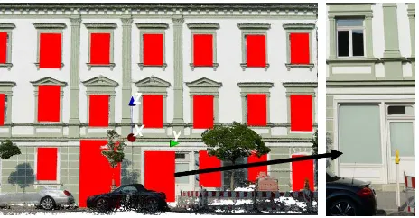
Figure 11: The left facade shows localized windows and doors (filled red polygons) of a facade. An image of a part of the facade is depicted on the right. The arrows shows a false localization of a door.
the strong hypotheses of window and door outlines generated through our combined angular-plane sweeping and boundary es-timation. Our algorithm requires no parameter fine tuning for a diversity of input data compared to image based methods for find-ing object boundaries e.g., the Canny edge detector. However, it will show a poor performance if the 3D geometry of off-the-facade objects is lacking, e.g., for modern off-the-facades with very huge glass windows embedded within the facade, popular for office buildings.
We analyze the overall performance of our algorithm on 20 data sets: 18 from image matching e.g., (Kuhn et al., 2013) and 2 from LiDAR with a point density of 0.01m. For the (dense) im-age matching, 20-80 imim-ages at 3264×2448 resolution were cap-tured using a RICOH Caplio 500SE camera in a wide baseline configuration. Table 2 summarizes the results of the number of true detections of windows and doors using the templates from the span. The poor detections of the doors from the point clouds from image matching is due to the occlusion of doors by cars parked in front of the buildings. Occlusion is also a problem for the lower windows. Additionally, the poor performance on the
Rectangular Template # objects correct wrong #windows(image matching) 645 580 65 #doors(image matching) 40 26 14 #windows(LiDAR) 35 34 1 #doors(LiDAR) 7 7 0 Half-Circular Template
#windows(image matching) 60 47 13 #doors(image matching) 34 26 8 #windows(LiDAR) 12 12 0 Arched-Dormer Template
#windows(image matching) 27 16 11 Gothic Template
#windows(image matching) 15 13 2
Table 2: Results of our experiments conducted on different data sets using the four templates for windows and doors. The number of correct versus wrong localizations for 20 data sets of point clouds of facades.
detections of the arched-dormer models is due to the difficulties to distinguish between the arched-dormer and the simple rectan-gular template.
3.1 Geometrical Evaluation
We count objects as true positives if and only if the enclosed polygon defining the localised outlines is having an overlap larger than 50%. We consider only rectangular windows from category Type-1 of Table 1 for this evaluation and substantiate our choice by the frequent occurrence of this window type and the ease of annotation of bounding boxes compared to spline curves. The primary reference data set used for the evaluation concerning geometrical accuracy are self annotated bounding boxes in 3D point clouds of facades acquired by matching images. We annotated 200 bounding boxes of rectangular shaped windows from 9 facades. For each of these facades, a dominant vertical plane was segmented. All annotated bounding boxes as well as the localized rectangular window outlines are projected on the dominant plane. Next, we computed for each localized outline the intersection over union area (Jaccard Index). On this criterion, we achieved a mean accuracy of 85% for all 200 annotated bounding boxes.
4 CONCLUSION
ACKNOWLEDGEMENTS
References
Akaike, H., 1973. Information Theory and an Extension of the Maximum Likelihood Principle. In: 2nd Intern. Symp. on In-formation Theory, pp. 267–281.
Alegre, F. and Dellaert, F., 2004. A Probabilistic Approach to the Semantic Interpretation of Building Facades. In: International Workshop on Vision Techniques Applied, pp. 1–12.
Becker, S. and Haala, N., 2008. Integrated LIDAR and Image Processing for the Modelling of Building Fa-cades. Photogrammetrie–Fernerkundung–Geoinformation 2008(2), pp. 65–81.
Brandenburger, W., Drauschke, M., Nguatem, W. and Mayer, H., 2013. Cornice Detection Using Facade Image and Point Cloud. Photogrammetrie–Fernerkundung–Geoinformation 2013(5), pp. 511–521.
Dick, A. R., Torr, P. H. S. and Cipolla, R., 2004. Modelling and Interpretation of Architecture from Several Images. Interna-tional Journal of Computer Vision 60(2), pp. 111–134.
Ferrari, V., Tuytelaars, T. and Van Gool, L., 2006. Object detec-tion by contour segment networks. In: Proceedings of the 9th European Conference on Computer Vision - Volume Part III, ECCV’06, Springer-Verlag, Berlin, Heidelberg, pp. 14–28.
Frahm, J.-M., Fite-Georgel, P., Gallup, D., Johnson, T., Raguram, R., Wu, C., Jen, Y.-H., Dunn, E., Clipp, B., Lazebnik, S. and Pollefeys, M., 2010. Building Rome on a Cloudless Day. In: ECCV, LNCS 6314, pp. 368–381.
Friedman, S. and Stamos, I., 2013. Online Detection of Repeated Structures in Point Clouds of Urban Scenes for Compression and Registration. International Journal of Computer Vision 102(1-3), pp. 112–128.
Fritsch, D., Becker, S. and Rothermel, M., 2013. Modeling Fa-cade Structures Using Point Clouds From Dense Image Match-ing. In: International Conference on Advances in Civil, Struc-tural and Mechanical Engineering, pp. 57–64.
Isard, M. and Blake, A., 1998. CONDENSATION: Conditional Density Propagation for Visual Tracking. International Journal of Computer Vision 29, pp. 5–28.
Kuhn, A., Hirschmueller, H. and Mayer, H., 2013. In: J. Weick-ert, M. Hein and B. Schiele (eds), GCPR, pp. 41–50.
Lafarge, F. and Mallet, C., 2012. Creating Large-Scale City Models from 3D-Point Clouds: A Robust Approach with Hy-brid Representation. International Journal of Computer Vision 99(1), pp. 69–85.
Lin, H., Gao, J., Zhou, Y., Lu, G., Ye, M., Zhang, C., Liu, L. and Yang, R., 2013. Semantic Decomposition and Reconstruction of Residential Scenes from LiDAR Data. ACM Transactions on Graphics 32(4), pp. 66:1–66:10.
Mayer, H., Bartelsen, J., Hirschm¨uller, H. and Kuhn, A., 2012. Dense 3D Reconstruction from Wide Baseline Image Sets. In: Outdoor and Large-Scale Real-World Scene Analysis - 15th International Workshop on Theoretical Foundations of Com-puter Vision, LNCS 7474, pp. 285–304.
Muja, M. and Lowe, D. G., 2009. Fast approximate nearest neigh-bors with automatic algorithm configuration. In: International Conference on Computer Vision Theory and Application VIS-SAPP’09), INSTICC Press, pp. 331–340.
Nguatem, W., Drauschke, M. and Mayer, H., 2012. Finding cuboid-based building models in point clouds. ISPRS XXXIX-B3, pp. 149–154.
Riemenschneider, H., Donoser, M. and Bischof, H., 2010. Us-ing partial edge contour matches for efficient object category localization.
Ripperda, N. and Brenner, C., 2006. Reconstruction of Fa-cade Structures Using a Formal Grammar and RjMCMC. In: DAGM 2006, LNCS 4174, pp. 750–759.
Rissanen, J., 1987. Minimum-Description-Length Principle. Wi-ley & Sons.
Rusu, R. B., Blodow, N., Marton, Z.-C., Soos, A. and Beetz, M., 2007. Towards 3d object maps for autonomous household robots. In: Proceedings of the 20th IEEE International Con-ference on Intelligent Robots and Systems (IROS), San Diego, CA, USA.
Schmittwilken, J., Yang, M. Y., F¨orstner, W. and Pl¨umer, L., 2009. Integration of Conditional Random Fields and Attribute Grammars for Range Data Interpretation of Man-Made Ob-jects. Annals of GIS 15(2), pp. 117–126.
Snavely, N., Seitz, S. M. and Szeliski, R., 2006. Photo Tourism: Exploring Photo Collections in 3D. ACM Transactions on Graphics 25(3), pp. 835–846.
Torr, P. H. S. and Zisserman, A., 2000. Mlesac: A new robust es-timator with application to estimating image geometry. Com-puter Vision and Image Understanding 78, pp. 2000.