Constructing parametric quadratic curves
Caiming Zhang∗;1, Fuhua (Frank) Cheng2
Department of Computer Science, University of Kentucky, Lexington, KY 40506, USA
Received 19 December 1997; received in revised form 25 August 1998
Abstract
Constructing a parametric spline curve to pass through a set of data points requires assigning a knot to each data point. In this paper we discuss the construction of parametric quadratic splines and present a method to assign knots to a set of planar data points. The assigned knots are invariant under ane transformations of the data points, and can be used to construct a parametric quadratic spline which reproduces parametric quadratic polynomials. Results of comparisons of the new method with several known methods are included. c1999 Elsevier Science B.V. All rights reserved.
Keywords:Parametric quadratic curve; Interpolation; Knots; Spline
1. Introduction
Since their introduction by Schoenberg in 1946 [14], spline functions have been widely used in many areas of scientic computation, engineering design, and CAD due to their good properties such as local control capability, small strain energy, and numerical stability. The rst property enables local modication of a spline function while the second one facilitates its geometric smoothness. Quadratic and cubic splines are the most frequently used splines in various applications.
In computer graphics, image processing, computer vision, pattern recognition, CAD, and many other elds, modeling the shape of an image or an object usually requires the technique of paramet-ric curve interpolation [4], i.e., constructing a parametparamet-ric curve that interpolates, or passes through, a given set of points, called interpolation points or data points. The parametric curve is usually constructed using a spline method. The resulting curve is then used as an approximation of the desired image or object. The data points should be selected in a way so that good approximation is guaranteed.
∗Corresponding author. E-mail: [email protected].
1
Supported by Ford.
2Supported by NSF (9722728), Ford and Honda.
this parametric polynomial. Hence, a key issue in spline curve interpolation is the selection of parametric knots.
Presently there are four popular methods in use for choosing knot locations, namely, uniform parametrization (uniform method), accumulated chord length method (chord length method), cen-tripetal model [10], and anely invariant parametrization method (Foley=Nielson method) [7, 11]. The chord length method [1, 3, 5, 6] seems to be the most widely used one. As far as reproduction degree is concerned, none of these methods provides a reproduction degree higher than one. A new approach recently proposed by Zhang et al. [15] (referred as the ZCM method) has a reproduction degree of two. A deciency of the chord length, centripetal, and ZCM methods is that the knots determined by these methods are not invariant under ane transformations of the data points. The uniform and the Foley=Nielson methods are invariant under ane transformations of the data points, but the uniform method is only suitable for data points which are evenly spaced.
This paper discusses the problem of constructing parametric quadratic splines, and proposes a method to choose knots for a set of planar data points. The selected knots are invariant under ane transformations of the data points. The quadratic spline constructed using the selected knots can reproduce a parametric polynomial of degree two.
The remaining part of this paper is arranged as follows. In Section 2, the equations that parametric quadratic splines are required to satisfy are discussed. A method to choose knots for a given set of planar points is given in Section 3. The comparison of the new method with the chord length method, the centripetal model, Foley=Nielson method and the ZCM method is performed in Section 4.
2. Constructing parametric quadratic spline
Let Pi= (xi; yi); i= 1;2; : : : ; n, be an ordered sequence of distinct, planar data points, and ti be
the knots to be determined. For i from 2 to n, let ti−1= (ti−1+ti)=2. ti, i= 1; : : : ; n−1, are called nodes. Furthermore, we set t0=t1 and tn=tn. The goal is to construct a parametric quadratic spline P(t) with the following properties:
1. P(t) is a parametric quadratic polynomial on each subinterval [ti−1;ti]; i= 1;2; : : : ; n;
2. P(t) is C1 continuous on [t 1; tn];
3. P(ti) =Pi; i= 1;2; : : : ; n.
Note that, for the specied knots, there are two additional degrees of freedom for constructing this quadratic spline.
Let Pi denote the value of P(t) at the node ti. The segment of the quadratic spline P(t) on the
subinterval [ti−1;ti] is denoted by Pi(t); i= 2;3; : : : ; n−1. Pi(t) is a quadratic polynomial passing
through Pi−1; Pi and Pi. Pi(t) can be put in Lagrange’s form as follows:
Pi(t) =
2(t−ti) ti+1−ti−1
2(t−t
i) ti−ti−1
( Pi−1−Pi) +
2(t−ti−1)
ti+1−ti
( Pi−Pi)
+Pi; (1)
From P′
for using Pi=hi as the unknowns instead of Pi is to ensure that the resulting matrix is diagonally
dominant). Two extra conditions are needed to solve this system of equations. One option in intro-ducing two extra conditions is shown below. First, for the subinterval [t0;t1], construct a parametric quadratic curve P1(t) that interpolates P1;P1 and P2 in Lagrange’s form, then from the requirement that P′
By constructing a parametric quadratic curve Pn(t) on the subinterval [tn−1;tn] that interpolates Pn−1;Pn−1 and Pn in Lagrange’s form, and then imposing the requirement that Pn′−1(tn−1) =Pn′(tn−1), constructed by (2)–(4) reproduces the original parametric quadratic polynomial.
3. Determining knot ti
According to (2), the knots ti; i= 1;2; : : : ; n, can be dened by
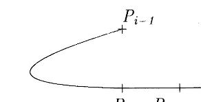
Fig. 1.Pi+2 is in the dotted region. where hi satisfy the condition
(1−si)hi−1=sihi (8)
with si dened in (2). Hence, the issue is how to determine si and hi, i= 1;2; : : : ; n−1. It will be
shown later that the techniques for constructing si and hi are invariant under ane transformation
of the data points.
3.1. Determining si
To be symmetrical, ve points Pj, i−26j6i+ 2, will be used to determine si. Suppose that Pi−1; Pi and Pi+1 are not collinear. Without loss of generality, we shall assume that the coordinates of the ve points are (xi−2; yi−2);(0;1);(0;0);(1;0) and (xi+2; yi+2) (see Fig. 1). Otherwise, simply apply a transformation similar to the one in [15] to transform them into the above forms.
For the four points Pi−1, Pi, Pi+1 and Pk with k being i−2 or i+ 2, let Ci(t) = (x(t); y(t)) be a
parametric cubic polynomial that passes through these points at the corresponding knots. By applying the parametric transformation
t=ti−1+ (ti+1−ti−1)s (9)
to Ci(t) = (x(t); y(t)), one changes the corresponding knots ti−1; ti; ti+1 and tk to 0; si;1 and k= (tk− ti−1)=(ti+1−ti−1), respectively, and changes Ci(t) to a function of s as follows:
x = x(s) =s(s−si) 1−si
+ (s)
(k)
xk−
k(k−si)
1−si
;
y = y(s) =(s−si)(s−1)
si
+ (s)
(k)
yk−
(k−si)(k−1) si
;
(10)
where
(s) =s(s−si)(s−1);
The construction of a quadratic curve which interpolates four planar points has been studied in [9, 12]. In the following we discuss the corresponding relations between the points and their parameters. If Pi−1; Pi; Pi+1 and Pk are points on a quadratic curve, then the cubic terms of (10) are zero, i.e.,
xk(1−si)−k(k−si) = 0; yksi−(k−si)(k−1) = 0:
(11)
Simple algebra shows that
(1−xk−yk)[(xk+yk)si2−2xksi] + (1−xk)xk= 0; k=xk+ (1−xk−yk)si: (12)
Eq. (12) has two roots. But only one can be used to dene si. If k equals i+ 2, from i+2= (ti+2−
ti−1)=(ti+1−ti−1)¿1 one gets the value of si, denoted by sir, as follows:
si=sir=
1
xi+2+yi+2
xi+2− s
xi+2yi+2
xi+2+yi+2−1 !
: (13)
It follows from (11) that the condition for 0¡si¡1 and i+2¿1 is
xi+2¿1 and yi+2¿0; (14)
i.e., (xi+2; yi+2) is in the dotted region of Fig. 1 and Theorem 2 follows.
Theorem 2. LetPj= (xj; yj); i−16j6i+ 2;be four planar data points;andP0 be the intersection of the line Pi−1Pi and the line Pi+1Pi+2. If P0 and Pi−1 are on dierent sides of PiPi+1; but Pi−1 and
Pi+2 are on the same side ofPiPi+1;thenPj; i−16j6i+2;determine a unique parametric quadratic polynomial that passes through these points successively.
In (12), if k equals i−2, then from the fact that i−2¡0 one gets the value of si, denoted by sil,
as follows:
si=sil=
1
xi−2+yi−2
xi−2+ s
xi−2yi−2
xi−2+yi−2−1 !
: (15)
The condition for 0¡si¡1 and i−2¡0 is
xi−2¿0 and yi−2¿1: (16)
By substituting (xi−2; yi−2) and (xi+2; yi+2) into (12), one gets two equations. The common root si
of these two equations, denoted by sm i , is
si=sim=
A(xi+2; yi+2)(xi−2+yi−2)−A(xi−2; yi−2)(xi+2+yi+2) 2xi+2yi−2−2xi−2yi+2
; (17)
where
A(x; y) = (1−x)x=(1−x−y):
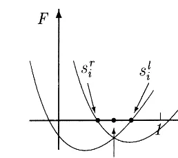
The geometric meaning ofsm
i is shown in Fig. 2 (where F= (1−xk−yk)[(xk+yk)si2−2xksi]+(1−xk)xk,
Fig. 2. Geometric meaning of sm i .
With these three possible values to dene si, one option is to form si as a linear combination of
(13), (15) and (17). These values have dierent inuences on the formation of si. The one close to
0.5 should have a bigger inuence than the ones close to 0 or 1. si is dened as follows:
si=
If the two quadratic curves shown in Fig. 2 have no intersection point in the interval [0;1], then
sm
cubic terms of (10) zero, then we determine si by minimizing the sum of the squared coecients
of the cubic terms, i.e., for k=i−2 or i+ 2, if we set H(si; k) is not unique. To remove this shortcoming, the following remedy is used. For the four
where
() =(−i)(−i+1):
The sum of the squared coecients of the cubic terms of (18) is
H1(i; i+1) =
The sum of the squared coecients of the cubic terms of (19) is
H2(i; i+1) =
The values of i and i+1 are determined by minimizing the following function:
H1(i; i+1) +H2(i; i+1): (20)
Fig. 3.Pi; Pi+1 and Pi+2 are nearly collinear.
The following illustration shows that this is a reasonable choice. Without loss of generality, we assume that Pj= (xj; yi); j=i−1; i; i+ 1. A quadratic polynomial (x(s); y(s)) passing through these
For the end points, (1) if the data points are not closed thens2corresponding toC2(s) is determined by (13) using four points Pj; j= 1;2;3;4, and similarly,sn−1 corresponding to Cn−1(s) is determined by (15); (2) if the data points are closed (P1=Pn) then a cyclic solution is used.
Note that if the last three points of Pi−1; Pi; Pi+1 and Pi+2 are nearly collinear, si dened by (13)
3.2. Determining hi
Although we have not seen unsatisfactory curves resulted from the above approach, it is obvious that hi and hj may have large dierence when j is much bigger than i.
Similar to [15], we recommend using two extra conditions h1 andhn−1 to solve the system. The re-maining unknowns h2; h3; : : : ; and hn−2 are determined by the least square method. Let
and re-arranging the terms, we obtain
If h1 and hn−1 are known, the solution of (24) is uniquely determined. One option in setting up
h1 and hn−1 is shown below. If the given data points are closed, i.e., (x1; y1) = (xn; yn), we simply
take h1=hn−1= 1. If the data points are not closed, h1 and hn−1 are determined by the following consideration: if Pi, i= 1;2; : : : ; n, are dened by (5), then h1 and hn−1 shall satisfy the following conditions:
t=t1+ (tn−1−t1)s
is applied to the four parameters corresponding to the four points, they become 0; s2;1 and n,
respectively, where s2 and n are dened by (13) and (12) or by (21) (h1=i, hn−1= 1−i+1). If
s2 and n are dened by (13) and (12), then h1 and hn−1 are taken as
h1=s2= (t2−t1)=(tn−1−t1);
hn−1=n−1 = (tn−tn−1)=(tn−1−t1);
(25)
and Theorem 3 follows.
Theorem 3. If the knots ti; i= 1;2; : : : ; n; dened by (23)–(25) and (7) are used to construct a quadratic spline using (2)–(4), then the constructed spline reproduces parametric quadratic polynomials.
Proof. It is sucient to prove that if the given data points Pi; i= 1;2; : : : ; n, are dened by (5),
then the determined ti; i= 1;2; : : : ; n, satisfy the following condition:
ti−ti−1=(ui−ui−1); i= 2;3; : : : ; n−2; (26)
for some ¿0. (25) shows = 1=(un−1−u1).
Our experiments show that if the data points are not closed, simply taking h1=hn−1= 1 also gives good results.
Theorem 4. The knots ti; i= 1;2; : : : ; n; dened by (7), (23) and (24) with the end conditions of setting h1 and hn−1 to (25), or simply to 1; are invariant under ane transformations of the data points.
Proof. It is sucient to prove that xi+2 and yi+2 in (13) are invariant under ane transformations of the data points. LetP1 be the projection of Pi+2 on the w axis along the v axis (see Fig. 1). Then
P1= (0; yi+2) and P0= (0; yi+2=(1−xi+2)). Thus
xi+2=
|P0P1|
|P0Pi|
; yi+2=
|PiP1|
|PiPi−1|
:
Since an ane transformation does not change the ratios of these segments, xi+2 and yi+2 are invariant.
H2(i; i+1). Specically, the coordinates of Pi−1; Pi; Pi+1 and Pi+2 are transformed into the form (x; y; z) = (0;1;0);(0;0;0);(1;0;0);(vi+2; wi+2;1), and H1(i; i+1) is dened as
H1(i; i+1) = 1
(1)2 "
vi+2−
i i+1(i+1−i)
2 +
wi+2−
(1)
ii+1 2
+ 1 #
:
H2(i; i+1) can be dened similarly.
4. Experiments
The new method has been implemented and compared with the chord length method, the centripetal model, the Foley=Nielson method and the ZCM method, where the ZCM and the new methods are the versions that reproduce quadratic polynomials. In the new method, in (21) is set to 0.1 for determining si; i= 2;3; : : : ; n−2, and set to 0.01 for determining h1 and hn−1. The comparison is performed on the quality of the parametric quadratic spline curves constructed using the knots determined by these methods. The chord length method is also used to determine knots in the construction of a cubic spline. The quadratic curve and cubic curve constructed by the chord length method are called chord2 and chord3, respectively.
Two types of data points are used to compare the quality of the methods. The rst type of data points is taken from two primitive curves. These data points are used to compare the approximation precision of the constructed spline curves. Another type of data points is taken from ([2, 3, 8, 10]). These data points are used to compare the shape of the constructed spline curves.
A knot computation method is considered to be better from the view point of approximation if the precision of the corresponding spline curve is better. The rst data points used in comparing the approximation precision are taken from the following primitive cubic curve: F(s) = (x(s); y(s)),
x=x(s) =s(s−1)(2s−1)K+ 3s2(3−2s);
y=y(s) =s(1−s)K;
where K= 1;2; : : : ;12.
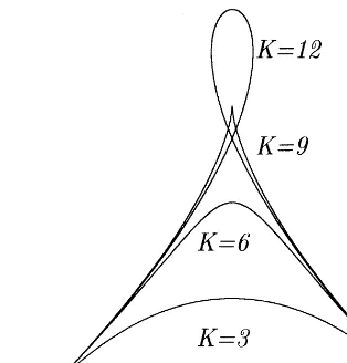
The cubic curve F(s) has the following properties: it is convex for K= 1;2;3;4, it has two inection points for K= 5;6;7;8, it has one cusp for K= 9, and it has one loop for K= 10;11;12. Note that when K= 3, the curve becomes y= 3x(1−x). For K= 3;6;9;12, the gures of F(s) on the region [0;1] are shown in Fig. 4.
The ve methods are compared on non-uniform data points generated by dividing the interval [0;1] into 20 subintervals using si dened as follows:
si= [i+sin (i∗(20−i))]=20; i= 0;1;2; : : : ;20; (27)
where 0660:25.
Fig. 4. Figures ofF(s) forK= 3;5;9;12. Table 1
Maximum absolute errors
Error chord2 chord3 centripetal Foley=Nielson ZCM New Exact
K= 1 7.52e−4 3.91e−4 1.22e−3 3.36e−4 1.96e−5 1.97e−5 9.98e−5
K= 2 1.20e−4 2.23e−5 1.11e−3 6.71e−4 1.19e−5 1.20e−5 4.88e−5
K= 3 7.95e−5 2.42e−5 1.61e−3 9.95e−4 3.30e−10 3.58e−10 3.30e−10
K= 4 1.08e−4 4.50e−5 2.05e−3 1.29e−3 2.34e−5 2.37e−5 5.10e−5
K= 5 1.97e−4 5.43e−5 2.36e−3 1.52e−3 4.04e−4 3.21e−4 1.03e−4
K= 6 5.67e−4 2.60e−4 2.35e−3 1.59e−3 5.68e−4 2.86e−4 1.55e−4
K= 7 1.95e−3 1.44e−3 1.68e−3 1.31e−3 9.34e−4 7.19e−4 2.08e−4
K= 8 4.90e−3 4.25e−3 1.41e−3 8.42e−4 4.07e−4 5.95e−4 2.61e−4
K= 9 8.52e−4 1.11e−3 1.91e−3 4.85e−4 5.84e−4 6.16e−4 3.14e−4
K= 10 6.69e−3 6.32e−3 2.41e−3 2.06e−3 4.99e−4 4.34e−4 3.67e−4
K= 11 3.78e−3 3.15e−3 3.41e−3 3.72e−3 4.33e−4 3.08e−4 4.20e−4
K= 12 1.91e−3 1.23e−3 5.04e−3 4.72e−3 4.19e−4 2.72e−4 4.74e−4
dened by
E(t) = min{|P(t)−F(s)|}
= min{|P˜i(t)−F(s)|; si
−16s6si}; i= 0;1;2; : : : ;19;
where P(t) is the spline curve constructed by one of the ve methods or the exact spline, ˜Pi(t) is
the segment of P(t) on the subinterval [ti−1; ti], and F(s) is the given primitive cubic curve.
When = 0:25 in (27), the maximum values of the error curve E(t) generated by the ve methods and the exact spline are shown in Table 1. When K= 3, F(s) is a quadratic polynomial, the ZCM and the new methods and the exact spline can reproduce it exactly. The errors 3.30e-10 and 3.58e-10 in Table 1 are caused by computing error of the computer.
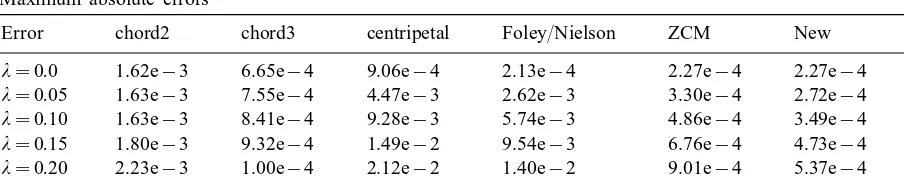
Table 2
Maximum absolute errors
Error chord2 chord3 centripetal Foley=Nielson ZCM New Exact
= 0:0 1.62e−3 6.65e−4 9.06e−4 2.13e−4 2.27e−4 2.27e−4 2.27e−4
= 0:05 1.63e−3 7.55e−4 4.47e−3 2.62e−3 3.30e−4 2.72e−4 2.81e−4
= 0:10 1.63e−3 8.41e−4 9.28e−3 5.74e−3 4.86e−4 3.49e−4 3.72e−4
= 0:15 1.80e−3 9.32e−4 1.49e−2 9.54e−3 6.76e−4 4.73e−4 4.81e−4
= 0:20 2.23e−3 1.00e−4 2.12e−2 1.40e−2 9.01e−4 5.37e−4 6.09e−4
= 0:25 2.75e−3 1.07e−3 2.84e−2 1.93e−2 1.16e−3 6.49e−4 7.58e−4
The theoretical derivation in Sections 2 and 3 shows that when used to assign knots in the construction of polynomial interpolants to data points whose signs in convexity are the same, the new method will reproduce parametric quadratic polynomials. Therefore, we have also compared the ve methods using data points taken from a convex elliptic curve:
x= 3 cos(2s); y= 2 sin(2s):
The interval [0;1] is also divided into 20 sub-intervals to dene data points. The maximum values of the error curve E(t) generated by the ve methods and the exact spline are shown in Table 2. Several methods for constructing quadratic splines to interpolate convex data points are available. The method presented in [13] can construct a visuallyC2 (G2) piecewise quadratic Bezier polynomial to interpolate convex data points.
Tables 1 and 2, as well as several other comparisons, show that (1) when the knots determined by the chord length method are used to construct splines, the resulting cubic curves have no obvious advantage in approximation precision over quadratic curves; (2) quadratic curves constructed by the new method generally have higher approximation precision than quadratic and cubic curves constructed by chord length method, as well as the ones constructed by the centripetal model and the Foley=Nielson method.
Finally, four sets of data points are used to compare the shape of the quadratic splines constructed by the ve methods. The four sets of data points are
(Akima;1970) {x; y}={(0;10);(2;10);(3;10);(5;10);(6;10);(8;10);(9;10:5);(11;15);
(12;50);(14;60);(15;85);
(Brodlie;1980) {x; y}={(0;1);(1;1:1);(2;1:1);(3;1:2);(4;1:3);(5;7:2);(6;3:1);(7;2:6);
(8;1:9);(9;1:7);(10;1:6)};
(Fritsch and Carlson;1980) {x; y}={(7:99;0);(8:09;2:76429e-5);(8:19;4:37498e-2);
(8:7;0:169183);(9:2;0:469428);(10;0:94374);(12;0:998636);(15;0:999919);(20;0:999994)}:
(Lee;1989); {x; y}={(0;0);(1:34;5);(5;8:66);(10;10);(10:6;10:4);(10:7;12);(10:7;28:6);
(10:8;30:2);(11:4;30:6);(19:6;30:6);(20:2;30:2)}:
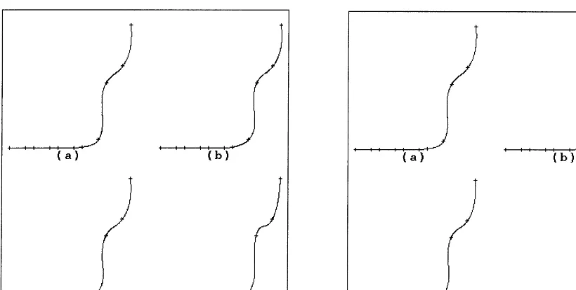
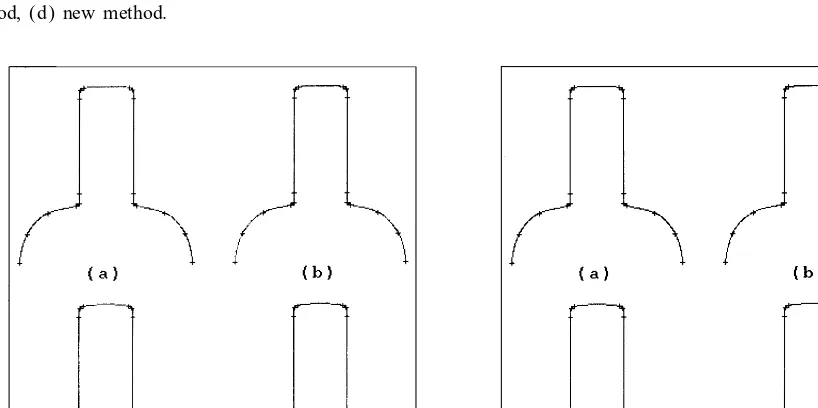
For the four sets of data points, the curves produced by the centripetal model, the Foley=Nielson method, the ZCM method and the new method are shown on the left hand side of Figs. 5–8. The curves on the right-hand side of Figs. 5–8 are interplants to the data points {vi; wi}, i= 1;2; : : : ;
produced by applying the following transformation to the four sets of data points,
Fig. 5. Data points taken from (Akima, 1970), (a) Foley=Nielson method, (b) centripetal model, (c) ZCM method, (d) new method.
Fig. 6. Data points taken from (Brodlie, 1980), (a) Foley=Nielson method, (b) centripetal model, (c) ZCM method, (d) new method.
Fig. 7. Data points taken from (Fritsch and Carlson, 1980), (a) Foley=Nielson method, (b) centripetal model, (c) ZCM method, (d) new method.
Fig. 8. Data points taken from (Lee, 1989), (a) Foley=Nielson method, (b) centripetal model, (c) ZCM method, (d) new method.
5. Conclusions
parametric cubic splines reproduce parametric cubic polynomials.
References
[1] J.H. Ahlberg, E.N. Nilson, J.L. Walsh, The Theory of Splines and their Applications, Academic Press, New York, 1967, p. 51.
[2] H. Akima, A new method of interpolation and smooth curve tting based on local procedures, J. ACM 17 (4) (1970) 589–602.
[3] K.W. Brodlie, A review of methods for curve and function drawing, in: K.W. Brodile (Ed.), Mathematical Methods in Computer Graphics and Design, Academic Press, London, 1980, p. 1.
[4] F. Cheng, B.A. Barsky, Interproximation: interpolation and approximation using cubic spline curves, Comput. Aided Design 23 (10) (1991) 700–706.
[5] C. de Boor, A Practical Guide to Splines, Springer, New York, 1978, p. 318.
[6] I.D. Faux, M.J. Pratt, Computational Geometry for Design and Manufacture, Ellis Horwood, Chichester, UK, 1979, p. 176.
[7] D.A. Foley, G.M. Nielson, Knot selection for parametric spline interpolation, in: T. Lyche, L.L. Schumaker (Eds.), Mathematical Methods in Computer Aided Geometric Design, Academic Press, New York, 1989, pp. 261–272. [8] F.N. Fritsch, R.E. Carlson, Monotone piecewise cubic interpolation, SIAM J. Numer. Anal. 17 (1980) 238–246. [9] M.A. Lachance, A.J. Schwartz, Four point parabolic interpolation, Comput. Aided Geom. Design 9 (1991) 143–149. [10] E.T.Y. Lee, Choosing nodes in parametric curve interpolation, Comput. Aided Design 21 (6) (1989) 363–370. [11] G.M. Nielson, D.A. Foley, A survey of applications of an ane invariant metric, in: T. Lyche, L.L. Schumaker
(Eds.), Mathematical Methods in Computter Aided Geometric Design, Academic Press, New York, 1989, pp. 445– 468.
[12] J. Peters, Interpolation regions for convex cubic curve segments, Adv. Comput. Math. 6 (1996) 87–96.
[13] R. Schaback, Interpolation with piecewise quadratic visuallyC2 Bezier polynomials, Comput. Aided Geom. Design
6 (1989) 219–233.
[14] I.J. Schoenberg, Contributions to the problem of application of equidistant data by analytic functions, Quart. Appl. Math. 4 (1946) 45–99.