Sage Beginner's Guide ebook free download

(1)

(2)

Sage

Beginner's Guide

Unlock the full potential of Sage for simplifying and

automating mathematical computing

Craig Finch

(3)

Sage

Beginner's Guide

All rights reserved. No part of this book may be reproduced, stored in a retrieval system, or transmitted in any form or by any means, without the prior written permission of the publisher, except in the case of brief quotations embedded in critical articles or reviews. Every effort has been made in the preparation of this book to ensure the accuracy of the information presented. However, the information contained in this book is sold without warranty, either express or implied. Neither the author, nor Packt Publishing, and its dealers and distributors will be held liable for any damages caused or alleged to be caused directly or indirectly by this book.

Packt Publishing has endeavored to provide trademark information about all of the companies and products mentioned in this book by the appropriate use of capitals. However, Packt Publishing cannot guarantee the accuracy of this information.

First published: May 2011

Production Reference: 1250411

Published by Packt Publishing Ltd. 32 Lincoln Road

Olton

Birmingham, B27 6PA, UK. ISBN 978-1-849514-46-0

www.packtpub.com

(4)

Credits

Author

Craig Finch

Reviewers

Dr. David Kirkby Minh Nguyen

Acquisition Editor Usha Iyer

Development Editor Hyacintha D'Souza

Technical Editor Ajay Shanker

Indexers Tejal Daruwale Rekha Nair

Project Coordinator Joel Goveya

Proofreaders Aaron Nash Mario Cecere

Graphics

Nilesh Mohite

Production Coordinator Adline Swetha Jesuthas

Cover Work

(5)

About the Author

Craig Finch

is a Ph. D. Candidate in the Modeling and Simulation program at the University of Central Florida (UCF). He earned a Bachelor of Science degree from the University of Illinois at Urbana-Champaign and a Master of Science degree from UCF, both in electrical engineering. Craig worked as a design engineer for TriQuint Semiconductor, and currently works as a research assistant in the Hybrid Systems Lab at the UCF NanoScience Technology Center. Craig's professional goal is to develop tools for computational science and engineering and use them to solve difficult problems. In particular, he is interested in developing tools to help biologists study living systems. Craig is committed to using, developing, and promoting open-source software. He provides documentation and "how-to" examples on his blog at http://www.shocksolution.com.

(6)

About the Reviewers

Dr. David Kirkby

is a chartered engineer living in Essex, England. David has a B.Sc. in Electrical and Electronic Engineering, an M.Sc. in Microwaves and OptoElectronics, and a Ph.D. in Medical Physics. Despite David's Ph.D. being in Medical Physics, it was primarily an engineering project, measuring the optical properties of human tissue, with a mixture of Monte Carlo modeling, radio frequency design, and laser optics. David was awarded his Ph.D. in 1999 from University College London.

Although not a mathematician, Dr. Kirkby has made extensive use of mathematical software. Most of his experience has been with MathematicaTM from Wolfram Research, although he has used both MATLABTM and SimulinkTM too.

David is the author of a number of open-source projects, including software for modeling transmission lines using finite difference (http://atlc.sourceforge.net/), design of

Yagi-Uda antennas (http://www.g8wrb.org/yagi/) which can use a genetic algorithm

for optimization, as well as software for data collection and analysis from electronic test equipment. David once wrote a web-based interface to MathematicaTM (http://witm. sourceforge.net/) which allows MathematicaTM to be used from a personal computer,

PDA or smartphone.

Soon after the Sage project was started by Professor William Stein, Dr. Kirkby joined the development of Sage. He primarily worked on the successful port of Sage to the Solaris and OpenSolaris operating systems and encourages other developers to write portable code, conforming to POSIX standard, avoiding GNUisms.

Professionally, David's skill sets include computer modeling, radio frequency design, analogue circuit design, electromagnetic compatibility and optics—both free space and integrated. David has also been a Solaris system administrator for the University of Washington where the Sage project is based.

When not working on writing software, David enjoys playing chess, gardening, and spending time with his wife Lin and dog Smudge.

(7)

(8)

www.PacktPub.com

Support files, eBooks, discount offers and more

You might want to visit www.PacktPub.com for support files and downloads related to

your book.

Did you know that Packt offers eBook versions of every book published, with PDF and ePub files available? You can upgrade to the eBook version at www.PacktPub.com and as a print

book customer, you are entitled to a discount on the eBook copy. Get in touch with us at

service@packtpub.com for more details.

At www.PacktPub.com, you can also read a collection of free technical articles, sign up for a

range of free newsletters and receive exclusive discounts and offers on Packt books and eBooks.

http://PacktLib.PacktPub.com

Do you need instant solutions to your IT questions? PacktLib is Packt's online digital book library. Here, you can access, read and search across Packt's entire library of books.

Why Subscribe?

Fully searchable across every book published by Packt Copy & paste, print and bookmark content

On demand and accessible via web browser

Free Access for Packt account holders

If you have an account with Packt at www.PacktPub.com, you can use this to access

(9)

(10)

Preface

1 Chapter 1: What Can You Do with Sage?

9

Getting started 9

Using Sage as a powerful calculator 12

Symbolic mathematics 14

Linear algebra 17

Solving an ordinary differential equation 18

More advanced graphics 19

Visualising a three-dimensional surface 20 Typesetting mathematical expressions 21

A practical example: analysing experimental data 22

Time for action – fitting the standard curve 22

Time for action – plotting experimental data 24

Time for action – fitting a growth model 25

Summary 26

Chapter 2: Installing Sage

29

Before you begin 29

Installing a binary version of Sage on Windows 30

Downloading VMware Player 30

Installing VMWare Player 30

Downloading and extracting Sage 30

Launching the virtual machine 31

Start Sage 32

Installing a binary version of Sage on OS X 33

Downloading Sage 34

Installing Sage 34

(11)

Table of Contents

[ ii ]

Installing a binary version of Sage on GNU/Linux 35

Downloading and decompressing Sage 35 Running Sage from your user account 36

Installing for multiple users 37

Building Sage from source 38

Prerequisites 38

Downloading and decompressing source tarball 39

Building Sage 39

Installation 39

Summary 39

Chapter 3: Getting Started with Sage

41

How to get help with Sage 41

Starting Sage from the command line 42

Using the interactive shell 43

Time for action – doing calculations on the command line 43

Getting help 45

Command history 46

Tab completion 47

Interactively tracing execution 48

Using the notebook interface 48

Starting the notebook interface 49

Time for action – doing calculations with the notebook interface 52

Getting help in the notebook interface 54

Working with cells 54

Working with code 55

Closing the notebook interface 55

Displaying results of calculations 56

Operators and variables 56

Arithmetic operators 57

Numerical types 58

Integers and rational numbers 58

Real numbers 59

Complex numbers 60

Symbolic expressions 60

Defining variables on rings 61

Combining types in expressions 62

Strings 62

Time for action – using strings 62

Callable symbolic expressions 63

Time for action – defining callable symbolic expressions 64

(12)

Table of Contents

[ iii ]

Functions 66

Time for action – calling functions 66

Built-in functions 68

Numerical approximations 68

The reset and restore functions 69

Defining your own functions 70

Time for action – defining and using your own functions 70

Functions with keyword arguments 72

Time for action – defining a function with keyword arguments 72

Objects 73

Time for action – working with objects 74

Getting help with objects 75

Summary 77

Chapter 4: Introducing Python and Sage

79

Python 2 and Python 3 79

Writing code for Sage 80

Long lines of code 81

Running scripts 81

Sequence types: lists, tuples, and strings 82

Time for action – creating lists 82

Getting and setting items in lists 85

Time for action – accessing items in a list 85

List functions and methods 87

Tuples: read-only lists 87

Time for action – returning multiple values from a function 87

Strings 89

Time for action – working with strings 90

Other sequence types 92

For loops 92

Time for action – iterating over lists 92

Time for action – computing a solution to the diffusion equation 94

List comprehensions 99

Time for action – using a list comprehension 99

While loops and text file I/O 101

Time for action – saving data in a text file 101

Time for action – reading data from a text file 103

While loops 105

Parsing strings and extracting data 105 Alternative approach to reading from a text file 106

If statements and conditional expressions 107

(13)

Table of Contents

[ iv ]

Time for action – defining and accessing dictionaries 108

Lambda forms 110

Time for action – using lambda to create an anonymous function 110

Summary 111

Chapter 5: Vectors, Matrices, and Linear Algebra

113

Vectors and vector spaces 113

Time for action – working with vectors 114

Creating a vector space 115

Creating and manipulating vectors 116

Time for action – manipulating elements of vectors 116

Vector operators and methods 117

Matrices and matrix spaces 118

Time for action – solving a system of linear equations 118

Creating matrices and matrix spaces 120 Accessing and manipulating matrices 120

Time for action – accessing elements and parts of a matrix 120

Manipulating matrices 122

Time for action – manipulating matrices 122

Matrix algebra 124

Time for action – matrix algebra 124

Other matrix methods 125

Time for action – trying other matrix methods 126

Eigenvalues and eigenvectors 127

Time for action – computing eigenvalues and eigenvectors 127

Decomposing matrices 129

Time for action – computing the QR factorization 129

Time for action – computing the singular value decomposition 131

An introduction to NumPy 133

Time for action – creating NumPy arrays 133

Creating NumPy arrays 134

NumPy types 135

Indexing and selection with NumPy arrays 136

Time for action – working with NumPy arrays 136

NumPy matrices 137

Time for action – creating matrices in NumPy 137

Learning more about NumPy 139

Summary 139

Chapter 6: Plotting with Sage

141

Confusion alert: Sage plots and matplotlib 141

(14)

Table of Contents

[ v ]

Plotting symbolic expressions with Sage 142

Time for action – plotting symbolic expressions 142

Time for action – plotting a function with a pole 144

Time for action – plotting a parametric function 146

Time for action – making a polar plot 147

Time for action – plotting a vector field 149

Plotting data in Sage 150

Time for action – making a scatter plot 150

Time for action – plotting a list 151

Using graphics primitives 153

Time for action – plotting with graphics primitives 153

Using matplotlib 155

Time for action – plotting functions with matplotlib 155

Using matplotlib to "tweak" a Sage plot 157

Time for action – getting the matplotlib figure object 158

Time for action – improving polar plots 159

Plotting data with matplotlib 161

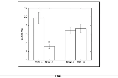
Time for action – making a bar chart 161

Time for action – making a pie chart 163

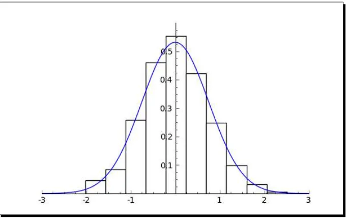
Time for action – plotting a histogram 164

Plotting in three dimensions 165

Time for action – make an interactive 3D plot 166

Higher quality output 167

Parametric 3D plotting 168

Time for action – parametric plots in 3D 168

Contour plots 169

Time for action – making some contour plots 169

Summary 171

Chapter 7: Making Symbolic Mathematics Easy

173

Using the notebook interface 174

Defining symbolic expressions 174

Time for action – defining callable symbolic expressions 174

Relational expressions 176

Time for action – defining relational expressions 176

Time for action – relational expressions with assumptions 178

Manipulating expressions 179

Time for action – manipulating expressions 179

Manipulating rational functions 180

Time for action – working with rational functions 181

(15)

Table of Contents

[ vi ]

Time for action – substituting symbols in expressions 182

Expanding and factoring polynomials 184

Time for action – expanding and factoring polynomials 184

Manipulating trigonometric expressions 186

Time for action – manipulating trigonometric expressions 186

Logarithms, rational functions, and radicals 187

Time for action – simplifying expressions 187

Solving equations and finding roots 190

Time for action – solving equations 190

Finding roots 191

Time for action – finding roots 191

Differential and integral calculus 193

Time for action – calculating limits 193

Derivatives 195

Time for action – calculating derivatives 195

Integrals 198

Time for action – calculating integrals 198

Series and summations 199

Time for action – computing sums of series 199

Taylor series 200

Time for action – finding Taylor series 200

Laplace transforms 202

Time for action – computing Laplace transforms 202

Solving ordinary differential equations 204

Time for action – solving an ordinary differential equation 204

Summary 206

Chapter 8: Solving Problems Numerically

207

Sage and NumPy 208

Solving equations and finding roots numerically 208

Time for action – finding roots of a polynomial 208

Finding minima and maxima of functions 210

Time for action – minimizing a function of one variable 210

Functions of more than one variable 211

Time for action – minimizing a function of several variables 211

Numerical approximation of derivatives 213

Time for action – approximating derivatives with differences 213

Computing gradients 215

Time for action – computing gradients 215

Numerical integration 217

(16)

Table of Contents

[ vii ]

Numerical integration with NumPy 219

Time for action – numerical integration with NumPy 219

Discrete Fourier transforms 220

Time for action – computing discrete Fourier transforms 220

Window functions 223

Time for action – plotting window functions 223

Solving ordinary differential equations 224

Time for action – solving a first-order ODE 224

Solving a system of ODEs 226

Time for action – solving a higher-order ODE 226

Solving the system using the GNU Scientific Library 229

Time for action – alternative method of solving a system of ODEs 229

Numerical optimization 231

Time for action – linear programming 231

Fitting a function to a noisy data set 233

Time for action – least squares fitting 233

Constrained optimization 235

Time for action – a constrained optimization problem 235

Probability 236

Time for action – accessing probability distribution functions 236

Summary 238

Chapter 9: Learning Advanced Python Programming

241

How to write good software 242

Object-oriented programming 243

Time for action – defining a class that represents a tank 244

Making our tanks move 249

Time for action – making the tanks move 249

Creating a module for our classes 253

Time for action – creating your first module 253

Expanding our simulation to other kinds of vehicles 258

Time for action – creating a vehicle base class 258

Creating a package for our simulation 263

Time for action – creating a combat simulation package 263

Potential pitfalls when working with classes and instances 268

Time for action – using class and instance attributes 269

Time for action – more about class and instance attributes 270

Creating empty classes and functions 272

Time for action – creating empty classes and functions 272

Handling errors gracefully 273

(17)

Table of Contents

[ viii ]

Exception types 278

Creating your own exception types 279

Time for action – creating custom exception types 279

Unit testing 284

Time for action – creating unit tests for the Tank class 284

Strategies for unit testing 288

Summary 289

Chapter 10: Where to go from here

291

Typesetting equations with LaTeX 291

Installing LaTeX 292

Time for action – PDF output from the notebook interface 293

The view function in the interactive shell 297 LaTeX mark-up in the notebook interface 297

Time for action – working with LaTeX markup in the notebook interface 297

Time for action – putting it all together 300

Speeding up execution 304

Time for action – detecting collisions between spheres 304

Time for action – detecting collisions: command-line version 307

Tips for measuring runtimes 309

Optimizing our algorithm 309

Time for action – faster collision detection 309

Optimizing with NumPy 311

Time for action – using NumPy 311

More about NumPy 314

Optimizing with Cython 314

Time for action – optimizing collision detection with Cython 314

Calling Sage from Python 316

Time for action – calling Sage from a Python script 316

Introducing Python decorators 319

Time for action – introducing the Python decorator 319

Making interactive graphics 322

Time for action – making interactive controls 322

Using interactive controls 328

Time for action – an interactive example 328

Summary 330

(18)

Preface

Results matter, whether you are a mathematician, scientist, or engineer. The time that you spend doing tedious mathematical calculations could be spent in more productive ways. Sage is an open-source mathematical software system that helps you perform many mathematical tasks. There is no reason to compute integrals or perform algebraic manipulations by hand when software can perform these tasks more quickly and accurately (unless you are a student who is learning these procedures for the first time). Students can also benefit from mathematical software. The ability to plot functions and manipulate symbolic expressions easily can improve your understanding of mathematical concepts. Likewise, it is largely unnecessary to write your own routines for numerical mathematics in low-level languages such as FORTRAN or C++. Mathematical software systems like Sage have highly optimized functions that implement common numerical operations like integration, solving ordinary differential equations, and solving systems of equations.

Sage is a collection of nearly 100 mathematical software packages, which are listed at

http://www.sagemath.org/links-components.html. When possible, existing tools

(19)

Preface

[ 2 ]

The mission statement of the Sage project is:

Creating a viable, free, open source alternative to Magma, Maple, Mathematica, and Matlab.

If you are familiar with any of these commercial mathematical software systems, then you already have a good idea what Sage does. Sage offers several advantages over its commercial competitors. Sage is free, open-source software, released under the GNU Public License version 2 or higher (GPLv2+). There is no cost to download and install Sage, whether you want to put it on your personal computer, install it in a university teaching lab, or deploy it on every workstation in a company. This advantage is especially important in developing countries. The GPL license also means that Sage is free, as in "freedom." There are no restrictions on how or where you use the software, the license can never be revoked, and there is no annual maintenance fee. Another advantage is that you have access to every line of source code, so you can see how every calculation is performed, and track exactly what changes are made from one version to the next. Unlike commercial software, the bug list for Sage is public, and it can be accessed at http://trac.sagemath.org/. Users are

encouraged to participate in the development of Sage by reporting and fixing bugs, and contributing new capabilities. With bugs and source code open for public review, you can have a high degree of confidence that Sage will produce correct results.

This book is written for people who are new to Sage, and perhaps new to mathematical software altogether. For this reason, the examples in the book emphasize undergraduate-level mathematics such as calculus, linear algebra, and ordinary differential equations. However, Sage is capable of performing advanced mathematics, and it has been cited in over 80

mathematical publications. A full list can be found at http://www.sagemath.org/library-publications.html. To benefit from this book, you should have some fundamental

knowledge of computer programming, but the Python language will be introduced as needed throughout the book. The next chapter will take you through some examples that showcase a small subset of Sage's capabilities.

What this book covers

Chapter 1, What can You do with Sage? covers how Sage can be used for: making simple

numerical calculations; performing symbolic calculations, solving systems of equations and ordinary differential equations; making plots in two and three dimensions; and analyzing experimental data and fitting models.

Chapter 2, Installing Sage covers how to install a binary version of Sage on Windows and

(20)

Preface

[ 3 ]

Chapter 3, Getting Started with Sage covers using the interactive shell; using the notebook

interface; learning more about operators and variables; defining and using callable symbolic expressions; calling functions and making simple plots; defining your own functions; and working with objects in Sage.

Chapter 4, Introducing Python and Sage covers how to: use lists and tuples to store

sequential data; iterate with loops; construct logical tests with "if" statements; read and write data files; and store heterogeneous data in dictionaries.

Chapter 5, Vectors, Matrices, and Linear Algebra covers how to create and manipulate vector

and matrix objects; how Sage can take the tedious work out of linear algebra; learning about matrix methods for computing eigenvalues, inverses, and decompositions; and getting started with NumPy arrays and matrices for numerical calculations.

Chapter 6, Plotting with Sage covers how to plot functions of one variable; making various

types of specialized 2D plots such as polar plots and scatter plots; using matplotlib to precisely format 2D plots and charts; and making interactive 3D plots of functions of two variables.

Chapter 7, Making Symbolic Mathematics Easy covers how to create symbolic functions

and expressions, and learn to manipulate them; solve equations and systems of equations exactly, and find symbolic roots; automate calculus operations like limits, derivatives, and integrals; create infinite series and summations to approximate functions; perform Laplace transforms; and find exact solutions to ordinary differential equations.

Chapter 8, Solving Problems Numerically covers how to find the roots of an equation;

compute integrals and derivatives numerically; find minima and maxima of functions; compute discrete Fourier transforms, and apply window functions; numerically solve an ordinary differential equation (ODE), and systems of ODEs; use optimization techniques to fit curves and find minima; and explore the probability tools in Sage.

Chapter 9, Learning Advanced Python Programming covers how to define your own classes;

use inheritance to expand the usefulness of your classes; organize your class definitions in module files; bundle module files into packages; handle errors gracefully with exceptions; define your own exceptions for custom error handling; and use unit tests to make sure your package is working correctly.

Chapter 10, Where to go from here covers how to export equations as PNG and PDF

(21)

Preface

[ 4 ]

What you need for this book

Required:

Sage

If using Windows, VMWare Player or VirtualBox is also required. Recommended, but not strictly necessary: LaTeX

Optional, for building Sage from source on Linux: GCC, g++, make, m4, perl,

ranlib, readline, and tar

Optional, for building Sage from source on OS X: XCode A web browser is required to use the notebook interface

Who this book is for

If you are an engineer, scientist, mathematician, or student, this book is for you. To get the most from Sage by using the Python programming language, we'll give you the basics of the language to get you started. For this, it will be helpful if you have some experience with basic programming concepts.

Conventions

In this book, you will find several headings appearing frequently.

To give clear instructions of how to complete a procedure or task, we use:

Time for action – heading

1.

_{Action 1}

2.

_{Action 2}

3.

_{Action 3}

Instructions often need some extra explanation so that they make sense, so they are followed with:

What just happened?

(22)

Preface

[ 5 ]

You will also find some other learning aids in the book, including:

Pop quiz – heading

These are short multiple choice questions intended to help you test your own understanding.

Have a go hero – heading

These set practical challenges and give you ideas for experimenting with what you have learned.

You will also find a number of styles of text that distinguish between different kinds of information. Here are some examples of these styles, and an explanation of their meaning. Code words in text are shown as follows: "We can use the help function to learn more

about it."

A block of code is set as follows:

print('This is a string') print(1.0)

print(sqrt)

Any command-line input or output is written as follows:

sage: R = 250e3 sage: C = 4e-6 sage: tau = R * C sage: tau

New terms and important words are shown in bold. Words that you see on the screen, in

menus or dialog boxes for example, appear in the text like this: "clicking the Next button moves you to the next screen".

Warnings or important notes appear in a box like this.

(23)

Preface

[ 6 ]

Reader feedback

Feedback from our readers is always welcome. Let us know what you think about this book—what you liked or may have disliked. Reader feedback is important for us to develop titles that you really get the most out of.

To send us general feedback, simply send an e-mail to feedback@packtpub.com, and

mention the book title via the subject of your message.

If there is a book that you need and would like to see us publish, please send us a note in

the SUGGEST A TITLE form on www.packtpub.com or e-mail suggest@packtpub.com.

If there is a topic that you have expertise in and you are interested in either writing or contributing to a book, see our author guide on www.packtpub.com/authors.

Customer support

Now that you are the proud owner of a Packt book, we have a number of things to help you to get the most from your purchase.

Downloading the example code

You can download the example code files for all Packt books you have purchased from your account at http://www.PacktPub.com. If you purchased this book elsewhere, you can

visit http://www.PacktPub.com/support and register to have the files e-mailed directly

to you.

Errata

Although we have taken every care to ensure the accuracy of our content, mistakes do happen. If you find a mistake in one of our books—maybe a mistake in the text or the code— we would be grateful if you would report this to us. By doing so, you can save other readers from frustration and help us improve subsequent versions of this book. If you find any errata, please report them by visiting http://www.packtpub.com/support, selecting

your book, clicking on the erratasubmissionform link, and entering the details of your

(24)

Preface

[ 7 ]

Piracy

Piracy of copyright material on the Internet is an ongoing problem across all media. At Packt, we take the protection of our copyright and licenses very seriously. If you come across any illegal copies of our works, in any form, on the Internet, please provide us with the location address or website name immediately so that we can pursue a remedy.

Please contact us at copyright@packtpub.com with a link to the suspected pirated material.

We appreciate your help in protecting our authors, and our ability to bring you valuable content.

Questions

You can contact us at questions@packtpub.com if you are having a problem with any

(25)

(26)

1

What Can You Do with Sage?

Sage is a powerful tool—but you don't have to take my word for it. This chapter will showcase a few of the things that Sage can do to enhance your work. At this point, don't expect to understand every aspect of the examples presented in this chapter. Everything will be explained in more detail in the later chapters. Look at the things Sage can do, and start to think about how Sage might be useful to you. In this chapter, you will see how Sage can be used for:

Making simple numerical calculations Performing symbolic calculations

Solving systems of equations and ordinary differential equations Making plots in two and three dimensions

Analysing experimental data and fitting models

Getting started

(27)

What Can You Do with Sage?

[ 10 ]

Go to http://www.sagenb.org/ and sign up for a free account. You can also browse

worksheets created and shared by others. If you have already installed Sage, launch the notebook interface by following the instructions in Chapter 3. The notebook interface

should look like this:

(28)

Chapter 1

[ 11 ]

Type in a name when prompted, and click Rename. The new worksheet will look like this:

(29)

[ 12 ]

Click the evaluate link or press Shift-Enter to evaluate the contents of the cell.

A new input cell will automatically open below the results of the calculation. You can also create a new input cell by clicking in the blank space just above an existing input cell. In

Chapter 3, we'll cover the notebook interface in more detail.

Using Sage as a powerful calculator

(30)

Chapter 1

[ 13 ]

If you have to make a calculation repeatedly, you can define a function and variables to make your life easier. For example, let's say that you need to calculate the Reynolds number, which is used in fluid mechanics:

You can define a function and variables like this:

Re(velocity, length, kinematic_viscosity) = velocity * length / kinematic_viscosity

v = 0.01 L = 1e-3 nu = 1e-6 Re(v, L, nu)

When you type the code into an input cell and evaluate the cell, your screen will look like this:

(31)

[ 14 ]

Sage can also perform exact calculations with integers and rational numbers. Using the pre-defined constant pi will result in exact values from trigonometric operations. Sage will even

utilize complex numbers when needed. Here are some examples:

Symbolic mathematics

Much of the difficulty of higher mathematics actually lies in the extensive algebraic manipulations that are required to obtain a result. Sage can save you many hours, and many sheets of paper, by automating some tedious tasks in mathematics. We'll start with basic calculus. For example, let's compute the derivative of the following equation:

The following code defines the equation and computes the derivative:

var('x')

f(x) = (x^2 - 1) / (x^4 + 1) show(f)

(32)

Chapter 1

[ 15 ]

The results will look like this:

The first line defines a symbolic variable x (Sage automatically assumes that x is always

a symbolic variable, but we will define it in each example for clarity). We then defined a function as a quotient of polynomials. Taking the derivative of f(x) would normally require the use of the quotient rule, which can be very tedious to calculate. Sage computes the derivative effortlessly.

Now, we'll move on to integration, which can be one of the most daunting tasks in calculus. Let's compute the following indefinite integral symbolically:

The code to compute the integral is very simple:

f(x) = e^x * cos(x)

f_int(x) = integrate(f, x) show(f_int)

The result is as follows:

To perform this integration by hand, integration by parts would have to be done twice, which could be quite time consuming. If we want to better understand the function we just defined, we can graph it with the following code:

(33)

[ 16 ]

Sage will produce the following plot:

Sage can also compute definite integrals symbolically:

To compute a definite integral, we simply have to tell Sage the limits of integration:

f(x) = sqrt(1 - x^2)

f_integral = integrate(f, (x, 0, 1)) show(f_integral)

The result is:

(34)

Chapter 1

[ 17 ]

Have a go hero

There is actually a clever way to evaluate the integral from the previous problem without doing any calculus. If it isn't immediately apparent, plot the function f(x) from 0 to 1 and see if you recognize it. Note that the aspect ratio of the plot may not be square.

The partial fraction decomposition is another technique that Sage can do a lot faster than you. The solution to the following example covers two full pages in a calculus textbook — assuming that you don't make any mistakes in the algebra!

f(x) = (3 * x^4 + 4 * x^3 + 16 * x^2 + 20 * x + 9) / ((x + 2) * (x^2 + 3)^2)

g(x) = f.partial_fraction(x) show(g)

We'll use partial fractions again when we talk about solving ordinary differential equations symbolically.

Linear algebra

Linear algebra is one of the most fundamental tasks in numerical computing. Sage has many facilities for performing linear algebra, both numerical and symbolic. One fundamental operation is solving a system of linear equations:

Although this is a tedious problem to solve by hand, it only requires a few lines of code in Sage:

A = Matrix(QQ, [[0, -1, -1, 1], [1, 1, 1, 1], [2, 4, 1, -2], [3, 1, -2, 2]])

(35)

[ 18 ]

The answer is as follows:

Notice that Sage provided an exact answer with integer values. When we created matrix A, the argument QQ specified that the matrix was to contain rational values. Therefore,

the result contains only rational values (which all happen to be integers for this problem).

Chapter 5 describes in detail how to do linear algebra with Sage.

Solving an ordinary differential equation

Solving ordinary differential equations by hand can be time consuming. Although many differential equations can be handled with standard techniques such as the Laplace transform, other equations require special methods of solution. For example, let's try to solve the following equation:

The following code will solve the equation:

var('x, y, v') y=function('y', x) assume(v, 'integer')

f = desolve(x^2 * diff(y,x,2) + x*diff(y,x) + (x^2 - v^2) * y == 0, y, ivar=x)

show(f)

The answer is defined in terms of Bessel functions:

It turns out that the equation we solved is known as Bessel's equation. This example

illustrates that Sage knows about special functions, such as Bessel and Legendre functions. It also shows that you can use theassume function to tell Sage to make specific assumptions

(36)

Chapter 1

[ 19 ]

More advanced graphics

Sage has sophisticated plotting capabilities. By combining the power of the Python programming language with Sage's graphics functions, we can construct detailed illustrations. To demonstrate a few of Sage's advanced plotting features, we will solve a simple system of equations algebraically:

var('x') f(x) = x^2

g(x) = x^3 - 2 * x^2 + 2

solutions=solve(f == g, x, solution_dict=True)

for s in solutions: show(s)

We used the keyword argument solution_dict=True to tell the solve function to return

the solutions in the form of a Python list of Python dictionaries. We then used a for loop

to iterate over the list and display the three solution dictionaries. We'll go into more detail about lists and dictionaries in Chapter 4. Let's illustrate our answers with a detailed plot:

p1 = plot(f, (x, -1, 3), color='blue', axes_labels=['x', 'y']) p2 = plot(g, (x, -1, 3), color='red')

labels = [] lines = [] markers = []

for s in solutions:

x_value = s[x].n(digits=3) y_value = f(x_value).n(digits=3)

(37)

[ 20 ]

y_value+0.5), color='black'))

lines.append(line([(x_value, 0), (x_value, y_value)], color='black', linestyle='--'))

markers.append(point((x_value,y_value), color='black', size=30))

show(p1+p2+sum(labels) + sum(lines) + sum(markers)) The plot looks like this:

We created a plot of each function in a different colour, and labelled the axes. We then used another for loop to iterate through the list of solutions and annotate each one. Plotting will

be covered in detail in Chapter 6.

Visualising a three-dimensional surface

Sage does not restrict you to making plots in two dimensions. To demonstrate the 3D capabilities of Sage, we will create a parametric plot of a mathematical surface known as the "figure 8" immersion of the Klein bottle. You will need to have Java enabled in your web browser to see the 3D plot.

var('u,v') r = 2.0

f_x = (r + cos(u / 2) * sin(v) - sin(u / 2) * sin(2 * v)) * cos(u)

(38)

Chapter 1

[ 21 ]

f_z = sin(u / 2) * sin(v) + cos(u / 2) * sin(2 * v) parametric_plot3d([f_x, f_y, f_z], (u, 0, 2 * pi), (v, 0, 2 * pi), color="red")

In the Sage notebook interface, the 3D plot is fully interactive. Clicking and dragging with the mouse over the image changes the viewpoint. The scroll wheel zooms in and out, and right-clicking on the image brings up a menu with further options.

Typesetting mathematical expressions

Sage can be used in conjunction with the LaTeX typesetting system to create publication-quality typeset mathematical expressions. In fact, all of the mathematical expressions in this chapter were typeset using Sage and exported as graphics. Chapter 10 explains how to use

(39)

[ 22 ]

A practical example: analysing experimental data

One of the most common tasks for an engineer or scientist is analysing data from an experiment. Sage provides a set of tools for loading, exploring, and plotting data. The following series of examples shows how a scientist might analyse data from a population of bacteria that are growing in a fermentation tank. Someone has measured the optical density (abbreviated OD) of the liquid in the tank over time as the bacteria are multiplying. We want to analyse the data to see how the size of the population of bacteria varies over time. Please note that the examples in this section must be run in order, since the later examples depend upon results from the earlier ones.

Time for action – fitting the standard curve

The optical density is correlated to the concentration of bacteria in the liquid. To quantify this correlation, someone has measured the optical density of a number of calibration standards of known concentration. In this example, we will fit a "standard curve" to the calibration data that we can use to determine the concentration of bacteria from optical density readings:

import numpy

var('OD, slope, intercept')

def standard_curve(OD, slope, intercept):

"""Apply a linear standard curve to optical density data""" return OD * slope + intercept

# Enter data to define standard curve

CFU = numpy.array([2.60E+08, 3.14E+08, 3.70E+08, 4.62E+08, 8.56E+08, 1.39E+09, 1.84E+09])

optical_density = numpy.array([0.083, 0.125, 0.213, 0.234, 0.604, 1.092, 1.141])

OD_vs_CFU = zip(optical_density, CFU) # Fit linear standard

std_params = find_fit(OD_vs_CFU, standard_curve, parameters=[slope, intercept],

variables=[OD], initial_guess=[1e9, 3e8], solution_dict = True)

for param, value in std_params.iteritems(): print(str(param) + ' = %e' % value) # Plot

data_plot = scatter_plot(OD_vs_CFU, markersize=20,

facecolor='red', axes_labels=['OD at 600nm', 'CFU/ml']) fit_plot = plot(standard_curve(OD, std_params[slope], std_params[intercept]), (OD, 0, 1.2))

(40)

Chapter 1

[ 23 ]

The results are as follows:

What just happened?

We introduced some new concepts in this example. On the first line, the statement import numpy allows us to access functions and classes from a module called NumPy. NumPy is

based upon a fast, efficient array class, which we will use to store our data. We created a NumPy array and hard-coded the data values for OD, and created another array to store values of concentration (in practice, we would read these values from a file) We then defined a Python function called standard_curve, which we will use to convert optical density

values to concentrations. We used the find_fit function to fit the slope and intercept

parameters to the experimental data points. Finally, we plotted the data points with the

scatter_plot function and the plotted the fitted line with theplot function. Note that we

had to use a function called zip to combine the two NumPy arrays into a single list of points

before we could plot them with scatter_plot. We'll learn all about Python functions

in Chapter 4, and Chapter 8 will explain more about fitting routines and other numerical

(41)

[ 24 ]

Time for action – plotting experimental data

Now that we've defined the relationship between the optical density and the concentration of bacteria, let's look at a series of data points taken over the span of an hour. We will convert from optical density to concentration units, and plot the data.

sample_times = numpy.array([0, 20, 40, 60, 80, 100, 120, 140, 160, 180, 200, 220, 240, 280, 360, 380, 400, 420, 440, 460, 500, 520, 540, 560, 580, 600, 620, 640, 660, 680, 700, 720, 760, 1240, 1440, 1460, 1500, 1560])

OD_readings = numpy.array([0.083, 0.087, 0.116, 0.119, 0.122, 0.123, 0.125, 0.131, 0.138, 0.142, 0.158, 0.177, 0.213, 0.234, 0.424, 0.604, 0.674, 0.726, 0.758, 0.828, 0.919, 0.996, 1.024, 1.066, 1.092, 1.107, 1.113, 1.116, 1.12,

1.129, 1.132, 1.135, 1.141, 1.109, 1.004, 0.984, 0.972, 0.952]) concentrations = standard_curve(OD_readings, std_params[slope], std_params[intercept])

exp_data = zip(sample_times, concentrations)

data_plot = scatter_plot(exp_data, markersize=20, facecolor='red', axes_labels=['time (sec)', 'CFU/ml'])

(42)

Chapter 1

[ 25 ]

What just happened?

We defined one NumPy array of sample times, and another NumPy array of optical density values. As in the previous example, these values could easily be read from a file. We used

the standard_curve function and the fitted parameter values from the previous example

to convert the optical density to concentration. We then plotted the data points using the

scatter_plot function.

Time for action – fitting a growth model

Now, let's fit a growth model to this data. The model we will use is based on the Gompertz function, and it has four parameters:

var('t, max_rate, lag_time, y_max, y0')

def gompertz(t, max_rate, lag_time, y_max, y0):

"""Define a growth model based upon the Gompertz growth curve""" return y0 + (y_max - y0) * numpy.exp(-numpy.exp(1.0 +

max_rate * numpy.exp(1) * (lag_time - t) / (y_max - y0))) # Estimated parameter values for initial guess

max_rate_est = (1.4e9 - 5e8)/200.0 lag_time_est = 100

y_max_est = 1.7e9 y0_est = 2e8

gompertz_params = find_fit(exp_data, gompertz, parameters=[max_rate, lag_time, y_max, y0], variables=[t],

initial_guess=[max_rate_est, lag_time_est, y_max_est, y0_est], solution_dict = True)

for param,value in gompertz_params.iteritems(): print(str(param) + ' = %e' % value)

The fitted parameter values are displayed:

Finally, let's plot the fitted model and the experimental data points on the same axes:

gompertz_model_plot = plot(gompertz(t, gompertz_params[max_rate], gompertz_params[lag_time], gompertz_params[y_max],

(43)

[ 26 ]

The plot looks like this:

What just happened?

We defined another Python function called gompertz to model the growth of bacteria

in the presence of limited resources. Based on the data plot from the previous example, we estimated values for the parameters of the model to use an initial guess for the fitting routine. We used thefind_fit function again to fit the model to the experimental data,

and displayed the fitted values. Finally, we plotted the fitted model and the experimental data on the same axes.

Summary

This chapter has given you a quick, high-level overview of some of the many things that Sage can do for you. Don't worry if you feel a little lost, or if you had trouble trying to modify the examples. Everything you need to know will be covered in detail in later chapters.

Specifically, we looked at:

Using Sage as a sophisticated scientific and graphing calculator Speeding up tedious tasks in symbolic mathematics

Solving a system of linear equations, a system of algebraic equations, and an

(44)

Chapter 1

[ 27 ]

Making publication-quality plots in two and three dimensions Using Sage for data analysis and model fitting in a practical setting

(45)

(46)

2

Installing Sage

Remember that you don't actually have to install Sage to start using it. You can start learning Sage by utilizing one of the free public notebook servers that can be found at http://www. sagenb.org/. However, if you find that Sage suits your needs, you will want to install a

copy on your own computer. This will guarantee that Sage is always available to you, and it will reduce the load on the public servers so that others can experiment with Sage. In addition, your data will be more secure, and you can utilize more computing power to solve larger problems. This chapter will take you through the process of installing Sage on various platforms.

In this chapter we shall:

Install a binary version of Sage on Windows and install a binary version of Sage on

OS X

Install a binary version of Sage on GNU/Linux Compile Sage from source

Before you begin

At the moment, Sage is fully supported on certain versions of the following platforms: some Linux distributions (Fedora, openSUSE, Red Hat, and Ubuntu), Mac OS X, OpenSolaris, and Solaris. Sage is tested on all of these platforms before each release, and binaries are always available for these platforms. The latest list of supported platforms is available at http:// wiki.sagemath.org/SupportedPlatforms. The page also contains information about

(47)

Installing Sage

[ 30 ]

When downloading Sage, the website attempts to detect which operating system you are using, and directs you to the appropriate download page. If it sends you to the wrong download page, use the "Download" menu at the top of the page to choose the correct platform. If you get stuck at any point, the official Sage installation guide is available at

http://www.sagemath.org/doc/installation/.

Installing a binary version of Sage on Windows

Installing Sage on Windows is slightly more involved than installing a typical Windows program. Sage is a collection of over 90 different tools. Many of these tools are developed within a UNIX-like environment, and some have not been successfully ported to Windows. Porting programs from UNIX-like environments to Windows requires the installation of Cygwin (http://www.cygwin.com/), which provides many of the tools that are standard

on a Linux system. Rather than attempting to port all of the necessary tools to Cygwin on Windows, the developers of Sage have chosen to distribute Sage as a virtual machine that can run on Windows with the use of the free VMWare Player. A port to Cygwin is in progress, and more information can be found at http://trac.sagemath.org/sage_trac/wiki/ CygwinPort.

Downloading VMware Player

The VMWare Player can be found at http://www.vmware.com/products/player/.

Clicking the Download link will direct you to a registration form. Fill out and submit the form. You will receive a confirmation email that contains a link that must be clicked to complete the registration process and take you to the download page. Choose Start Download

Manager, which downloads and runs a small application that performs the actual download

and saves the file to a location of your choice.

Installing VMWare Player

After downloading VMWare Player, double-click the saved file to start the installation wizard. Follow the instructions in the wizard to install the Player. You will have to reboot the computer when instructed.

Downloading and extracting Sage

Download Sage by following the Download link from http://www.sagemath.org. The

(48)

Chapter 2

[ 31 ]

Launching the virtual machine

Launch VMware Player and accept the license terms. When the Player has started, click Open a Virtual Machine and select the Sage virtual machine, which is calledsage-vmware.vmx. Click

Play virtual machine to run Sage. If you have run Sage before, it should appear in the list of virtual machines on the left side of the dialog box, and you can double-click to run it.

(49)

Installing Sage

[ 32 ]

Start Sage

Once the virtual machine is running, you will see three icons. Double-clicking the Sage

Notebook icon starts the Sage notebook interface, while the Sage icon starts the

command-line interface. The first time you run Sage, you will have to wait while it regenerates files. When it finishes, you are ready to go.

(50)

Chapter 2

[ 33 ]

When you are done using Sage, choose Shut Down… from the System menu at the top of the

window, and a dialog will appear. Click the Shut Down button to close the virtual machine.

Installing a binary version of Sage on OS X

(51)

Installing Sage

[ 34 ]

Downloading Sage

Download Sage by following the Download link from http://www.sagemath.org. The site

should automatically detect that you are using OS X, and direct you to the right download page. Choose a mirror site close to you. Select your architecture (Intel for new Macs, or PowerPC for older G4 and G5 macs). Then, click the link for the correct .dmg file for you

version of Mac OS X. If you aren't sure, click the Apple menu on the far left side of the menu bar and choose About This Mac.

Installing Sage

Once the download is complete, double-click the .dmg file to mount the disk image. Drag

the Sage folder from the disk image to the desired location on your hard drive (such as the

Apps folder).

If the copy procedure fails, you will need to do it from the command line. Open the Terminal application and enter the following commands. Be sure to change the name sage-4.5-OSX-64bit-10.6-i386-Darwin.dmg to the name of the file you just downloaded:

$ cd /Applications

$ cp -R -P /Volumes/sage-4.5-OSX-64bit-10.6-i386-Darwin.dmg /sage .

After the copy process is complete, right-click on the icon for the disk image, and choose

Eject.

Starting Sage

Use the Finder to visit the Sage folder that you just created. Double-click on the icon called

Sage. It should open with the Terminal application. If it doesn't start, right-click on the icon,

go to the Open With submenu and choose Terminal.app. The Sage command line will

(52)

Chapter 2

[ 35 ]

There are three ways to exit Sage: type exit or quit at the Sage command prompt, or press

Ctrl-D in the Terminal window. You can then quit the Terminal application.

Installing a binary version of Sage on GNU/Linux

As with Mac OS X, you have the option of installing a pre-built binary application for your version of Linux, or downloading the source code and compiling Sage yourself. The same trade-offs apply to Linux. Keep in mind that the Sage team only distributes pre-build binaries for a few popular distributions. If you are using a different distribution, you'll have to compile Sage from source anyway. The following instructions will assume you are downloading a binary application. I will use Ubuntu as an example, but other versions of Linux should be very similar.

Most modern Linux distributions use a package manager to install and remove software. Sage is not available as an officially supported package for any Linux distribution at this time. "Unofficial" packages have been created for Debian, Mandriva, Ubuntu, and possibly others, but they are unlikely to be up to date and may not work properly. An effort to integrate Sage with Gentoo Linux can be found at https://github.com/cschwan/sage-on-gentoo.

Downloading and decompressing Sage

Download the appropriate pre-built binary from http://www.sagemath.org/download-linux.html. Choose the closest mirror, and then choose the appropriate architecture for

your operating system. If you're not sure whether your operating system is built for 32 or 64 bit operation, open a terminal and type the following on the command line:

$ uname –m

If the output contains 64, then your system is probably a 64-bit system. If not, it's a 32-bit. An alternative way to check is with the following command:

$ file /usr/bin/bin

(53)

Installing Sage

[ 36 ]

Once the download is done, uncompress the archive. You can use the graphical archiving tool for your version of Linux (the Ubuntu archiver is shown in the following screenshot). If you prefer the command line, type the following:

tar --lzma -xvf sage-*...tar.lzma

Running Sage from your user account

After decompression, you will have a single directory. This directory is self-contained, so no further installation is necessary. You can simply move it to a convenient location within your home directory. This is a good option if you don't have administrator privileges on the system, or if you are the only person who uses the system. To run Sage, open a terminal and change to the Sage directory (you will have to modify the command below, depending on the version you installed and where you installed it):

cfinch@ubuntu:$ cd sage-4.5.3-linux-32bit-ubuntu_10.04_lts-i686-Linux

Run Sage by typing the following:

cfinch@ubuntu:$ ./sage

(54)

Chapter 2

[ 37 ]

There are three ways to exit Sage: typeexit or quit at the Sage command prompt, or press

Ctrl-D in the terminal window.

Installing for multiple users

If you are the administrator of a shared system, you may want to install Sage so that everyone can use it. Since Sage consists of one self-contained directory, I suggest moving it

to the /opt directory:

sudo mv sage-4.5.3-linux-32bit-ubuntu_10.04_lts-i686-Linux /opt [sudo] password for cfinch:

To make it easy for everyone to run Sage, make a symbolic link from /usr/bin to the actual

location:

cfinch@ubuntu:/usr/bin$ sudo ln -s /opt/sage-4.5.3-linux-32bit-ubuntu_10.04_lts-i686-Linux/sage sage

[sudo] password for cfinch:

(55)

Installing Sage

[ 38 ]

Building Sage from source

This section will describe how to build Sage from source code on OS X or Linux. Although Sage consists of nearly 100 packages, the build process hides much of the complexity. It is impossible to provide instructions for all of the platforms that can build Sage, but the following guidelines should cover most cases. The official documentation for building Sage from source is available at http://sagemath.org/doc/installation/source.html.

Prerequisites

In order to compile Sage, you will need about 2.5GB of free disk space, and the following tools must be installed:

GCC

g++

gfortran

make

m4

perl ranlib tar

readline and its development headers

ssh-keygen (only needed to run the notebook in secure mode) latex (highly recommended, though not strictly required)

If you are running OS X (version 10.4 or later), install XCode to get all of these tools. XCode is available for free when you sign up as a developer at http://developer.apple.com/.

Make sure that you have XCode version 2.4 or later.

If you are running Linux, use your package manager to install any missing tools. For example, on a Debian-based system like Ubuntu, run the following on the command line:

$ sudo apt-get install build-essential m4 gfortran $ sudo apt-get install readline-common libreadline-dev

To install LaTeX (optional):

(56)

Chapter 2

[ 39 ]

Downloading and decompressing source tarball

Download the latest source tarball from http://sagemath.org/download-source. html. Open a terminal, change to the directory where you saved the tarball, and

decompress it with the following command:

$ tar -xvf sage-*.tar

Building Sage

If you have a multi-core or multi-processor machine, you can speed up the build process by performing a parallel compilation. You can control this by setting theMAKE environment

variable. For example, using Bash syntax, you can set the MAKE variable to use four cores:

$ export MAKE="make -j4"

Change to the Sage directory:

$ cd sage-*

Build Sage:

$ make

Sage may take a long time (1 hour to several days) to compile, depending on the speed of the machine.

Installation

When the compilation process is done, you should be able to run Sage from the build directory. If you want to move the Sage installation or make it available to other users on a shared Linux system, follow the directions in the previous sections.

Summary

(57)

(58)

3

Getting Started with Sage

In this chapter, you will learn the basic ideas that will be the foundation for using all the features of Sage. We will start by learning how to use the command line and notebook interfaces efficiently. Then, we'll look at basic concepts like variables, operators, functions, and objects. By the end of the chapter, you should be able to use Sage like a sophisticated scientific graphing calculator.

Using the interactive shell Using the notebook interface

Learning more about operators and variables Defining and using callable symbolic expressions Calling functions and making simple plots Defining your own functions

Working with objects in Sage

How to get help with Sage

The Sage documentation is accessible from the interactive shell and the notebook interface. Further help is available on the Web. The main Sage documentation page at http://www. sagemath.org/help.html provides links to dozens of resources. A few of these links are

especially useful:

The official Sage tutorial can be found at http://www.sagemath.org/doc/ tutorial/, and it is also accessible from the Help link in the notebook interface.

The Python language tutorial at http://docs.python.org/tutorial/ will also

be helpful.

The reference manual at http://www.sagemath.org/doc/reference/

(59)

Getting Started with Sage

[ 42 ]

Thematic tutorials athttp://www.sagemath.org/doc/thematic_tutorials/ index.html focus on specific topics.

The "Constructions" document athttp://www.sagemath.org/doc/ constructions/index.html describes how to do specific things with Sage.

Interactive resources, including mailing lists, an IRC channel, and a discussion forum are available if you get stuck. A complete list of these resources can be found at http://www. sagemath.org/development.html. The mailing lists sage-support and sage-devel are

intended for general questions. Other lists are available to discuss more specific topics.

Starting Sage from the command line

In the previous chapter, we learned how to start Sage. If you want to pass options to Sage when it starts, you can do so with command line arguments.

1. On OS X or a UNIX-like platform, start by opening a terminal window. On Windows, start the virtual machine and double-click the Terminal icon.

2. If you have added the Sage application directory to the PATH environment variable, you can just type sage at the command prompt. If not, you will need to enter the full

path to the Sage binary.

3. Add command line arguments, separated by spaces, and press Enter. For example, type the following at the command prompt to start Sage and automatically launch the notebook interface:

$ /Applications/sage/sage -notebook

There are many command line arguments, but you probably won't need them right away. Three of the most useful arguments are as follows:

Argument Description

(60)

Chapter 3

[ 43 ]

Using the interactive shell

The interactive shell provides a command-line interface to Sage. When you are done using Sage, remember to typequit or exit at the Sage prompt, or press Ctrl-D, to exit the

interactive shell. In the following examples, lines which start with the Sage command prompt

sage: indicate commands that you need to type in. Lines without the prompt indicate output

from Sage. Although most of the examples in this book utilize the notebook interface, they will work in the interactive shell, unless noted otherwise.

Time for action – doing calculations on the command line

Let's say that you need to make some quick calculations to design a simple electrical circuit. We will use the example of a series RC circuit, which consists of a resistor and a capacitor connected in series:

The voltage across the capacitor can be described by a linear, first-order differential equation. Eventually we will learn to solve differential equations with Sage, but for now we will just use the solution, which is well known:

1.

_{Define variables.}

First, we'll define some variables to work with. Type in the following text at the command prompt, and press Enter after every line:

sage: R = 250e3 sage: C = 4e-6 sage: tau = R * C sage: tau