Tarun Jain is an assistant professor of economics and public policy at the Indian School of Business. The author thanks Leora Friedberg, Sanjay Jain, and John Pepper for guidance and support. He is grateful to the Bankard Fund for Political Economy for fi nancial support and to Mark Rosenzweig and Andrew Foster for sharing the REDS data set. The data used in this article can be obtained October 2014 through September 2017 from Tarun Jain, AC8 Room 8119, Indian School of Business, Hyderabad AP India, Email: tj9d@virginia .edu.
[Submitted March 2012; accepted March 2013]
ISSN 0022- 166X E- ISSN 1548- 8004 © 2014 by the Board of Regents of the University of Wisconsin System
T H E J O U R N A L O F H U M A N R E S O U R C E S • 49 • 2
Fertility Behavior and Sex Bias in Large
Families
Tarun Jain
A B S T R A C T
This paper demonstrates that the social institutions of lineage maintenance, patrilocality, and joint families have a signifi cant role in explaining sex differences in survival and health outcomes in rural India. Tests using panel data from rural households support this explanation, which accounts for 7 percent of excess female mortality in Haryana and Rajasthan and 4 percent in Punjab. An institutional explanation suggests limits on the role for public policy in addressing large sex differences in health and mortality outcomes.
I. Introduction
Much of the existing literature suggests that parents actively discriminate in favor of boys through sex- selective feticide and infanticide, as well as differences in provi-sion of food and healthcare.1 However, the evidence suggests that these explanations are incomplete because the estimated number of excess female deaths due to feti-cide or infantifeti-cide do not account for the observed sex ratio (Dreze and Sen 2002). Despite arguments that parents actively discriminate against daughters in allocating nutrition and health resource, tests of intra- household allocation using recent data fail to reveal signifi cant bias in behavior (Griffi ths et al 2002). Instead, Basu (1989) and Arnold, Choe, and Roy (1998) present evidence that son- preference manifests itself predominantly in fertility behavior so that the resulting family structure is unfavorable to girls. Jensen (2003) argues that this fertility behavior takes the form of “stopping rules” where parents have children until a certain number of boys are born. Under such rules, the average girl in the population will have systematically more siblings than the average boy, leading to lower resource allocation and poorer outcomes even with equitable parent behavior in distribution. Rosenblum (2013) and Barcellos, Carvalho, and Lleras- Muney (2013) estimate that stopping rules have a signifi cant impact on differential outcomes for girls compared to boys. The fi rst contribution of this paper is to propose a plausible explanation for the origin of these stopping rules.
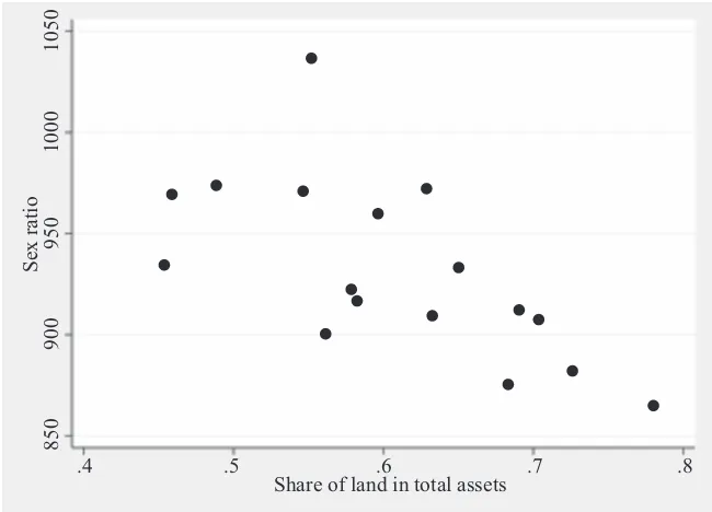
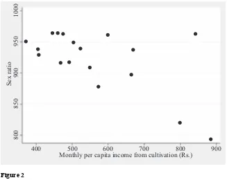
Another line of evidence suggests that sex imbalances are not uniform across all households. Rosenzweig and Schultz (1982) argue that discrimination against girls is driven by asymmetry in the economic or social marketplace, which would sug-gest that the worst outcomes should be observed in the most destitute families where the marginal value of an additional son is greatest. However, Census and National Sample Survey data shows the sex ratio is worse in Indian states such as Punjab and Haryana where land forms a large part of family assets (Figure 1) and where income from agriculture is high (Figure 2). Mahajan and Tarozzi (2007) report that gender differences in nutrition and health outcomes increased in the 1990s, a period of rapid
economic growth. Das Gupta (1987) as well as Chakraborty and Kim (2010) fi nd
that the difference between girls and boys is greater in middle class and higher caste households compared to lower- class and lower- caste households. If economic consid-erations drive discriminatory behavior, why are outcomes for girls relatively worse in agriculturally productive regions and among comparatively prosperous households? Addressing these contradictory fi ndings is the second contribution of this paper.
Household level data investigated in this paper indicates that girls experience worse mortality outcomes in large, multigenerational families known as “joint” families, which are common in rural farming communities. Caldwell, Reddy, and Caldwell’s (1984) framework sheds light on various family structures in India. A “nuclear fam-ily” is formed when a couple leaves their parents’ home upon marriage to form a
household with their unmarried, typically minor, children. In a “stem family,” two married couples cohabit in a household together. The younger husband is the son of the older couple. Finally, a “joint- stem family” refers to a family where an older patri-arch and his wife live with two or more adult sons, along with their wives and minor children.2 In the Rural Economic and Demographic Survey (REDS 1999), the child sex ratio was 0.816 girls per boy in joint families, compared to 0.912 girls otherwise. Why this would be is not clear because recent research has shown that children in joint families benefi t from higher levels of public good provision (Edlund and Rahman 2005). Proposing an explanation that is consistent with worse outcomes for girls in joint families is the third contribution of this paper.
I construct a model of bequest and fertility behavior among rural, land- owning fam-ilies in a patrilocal society. In most regions of India, adult daughters leave their natal family at the time of marriage for their husband’s home, and are considered members only of their family of marriage. Consequently, they rarely receive inheritances in the form of land because any land given to them would be lost to the family lineage
2. In this paper, I use “independent family” instead of nuclear family, and “joint family” as shorthand for a joint- stem family. Additionally, I differentiate between a “family” and “household” in the data, so co-residence within the household is not a requirement for membership of a joint or stem family.
Figure 1
Importance of land versus sex ratio
Source: Government of India (1998) and Census of India (2001)
Share of land in total assets
.4 .5 .6 .7 .8
850
900
950
1000
1050
(Agarwal 1998). The joint family head divides the land bequest among the remaining claimants, who are his adult sons. While doing so, the head will attempt to retain land within the family line carried through by his male descendants.
Why is land preservation so important in an agricultural society, particularly com-pared to more liquid assets such as cash or those that are more directly consumed such as livestock? First, land is a fi xed, immovable asset that cannot be lost or sto-len. Thus, unlike wage employment, land offers a source of permanent income either through sale or direct consumption of the product. This has important consequences in a society with little formal social insurance. For example, Rose (1999) reports that controlling for size of asset holdings, child survival outcomes are signifi cantly better in land- owning families. Second, farmers who cultivate their own land do not face classic agency problems and are motivated to exert maximum effort into production (Banerjee, Gertler, and Ghatak 2002). Third, the advantages of land compared to other types of assets are recognized by other agents in the village economy. For example, Feder and Onchan (1987) show that land ownership improves access to credit, even if it is not directly linked to farm investments. These reasons suggest that well- being of the lineage is symbiotic with preservation of land. Indeed, in a pioneering study of Indian villages, Srinivas (1976) wrote, “A man was acquiring land not only for himself but for his descendants . . . while a man may have had his descendants in mind when
Figure 2
Agricultural income versus sex ratio
Source: Government of India (1998) and Census of India (2001)
Monthly per capita income from cultivation (Rs.)
400 500 600 700 800 900
800
850
900
950
1000
buying land he also knew it would be divided after his death . . . but even worse than division of land among descendants was not having any. That meant the end of the lineage, a disaster which no one liked even to contemplate.”
Land possession, control, and preservation are signifi cant factors infl uencing behav-ior within rural families. With land sales rare, most families obtain land through in-heritance. The Hindu Succession Act (1956) specifi es that land acquired by inheritance should be divided equally among surviving sons, whereas property acquired separately can be distributed according to the head’s preferences. Nonetheless, implementation of the law might not be absolute, and adult sons have incentive to alter their behavior to get larger shares of land. If a head has only daughters, then the land passes from the head’s family to the daughter’s husband’s family and leaves the lineage. Thus, the household head might make land bequest decisions after observing how many sons his sons have because bequeathing land to a son with many daughters and few sons increases the probability that land will eventually leave the lineage. Claimants an-ticipate the head’s preferences and simultaneously make fertility choices to maximize their expected inheritance, taking into account expectations of other claimants’ fertil-ity choices. Thus, a claimant has greater incentive to try to have another child when the other claimants have more boys, and lower incentive to try to have another child when the other claimants have more girls, a prediction I term “strategic fertility.” An implication of this fertility pattern is that the average girl in a joint family has more siblings than the average boy, which has been shown to lead to worse health and sur-vival outcomes even when parents’ total resources are equitably distributed between their sons and daughters.
In this paper, I test for strategic bequest and fertility behavior as well as the demo-graphic implications of the hypothesis using a nationally representative panel data set of rural households in India. I fi nd that more sons for claimants are associated with larger shares of land bequests. Motivated by a desire to increase their inheritance, I expect that claimants in joint families will have a differential fertility response to the other claimants’ family structure, increasing fertility when the other claimants have more sons, and decreasing fertility when other claimants have more daughters. This implies that in the empirical model, the fertility response to the other claimants’ sons less the other claimants’ daughters is positive and signifi cant. In the sample with claimants from all joint families, I fi nd statistically signifi cant evidence of this differ-ential response, which is driven by large declines in fertility behavior when the other claimants have an additional daughter rather than increase in fertility when the other claimants have additional sons.
I also conduct two subsample analyses. First, I compare claimants in joint families (when the head is alive and the land has not yet been distributed) to claimants who have formed independent families after the head’s death. While the absolute differ-ence in the fertility response to the other claimants’ boys and girls is larger among the joint families compared to independent families, this difference is not statistically signifi cant for either family type. Second, I compare claimants in joint families that own land, where I expect strategic fertility to be salient, to those that do not. I fi nd that the difference in the fertility response to the other claimants’ boys and girls is positive and signifi cant in both types of families, perhaps because landless families mimic behavior of landowning families.
family with two or more claimants has nearly twice as many excess siblings compared to the average girl who is born in a multigenerational family with a single claimant. I calculate that approximately 7 percent of excess female mortality among joint families in Haryana and Rajasthan can be explained by this model. These results suggest an important but as yet unexamined role for household structure in explaining fertility behavior and poorer outcomes for girls. Thus, this paper contributes to an emerg-ing literature that recognizes the different forms of nonunitary households and family structures observed in developing countries. The joint family literature in particular is sparse, and this paper is one of few papers that incorporates inter- and intragen-erational dynamics within such families (Rosenzweig and Wolpin 1985; Foster and Rosenzweig 2002; Edlund and Rahman 2005).
This paper also adds to the strategic bequest literature pioneered by Bernheim, Shle-ifer, and Summers (1985). Because land bequests form a major share of wealth acqui-sition in agricultural societies, this framework is particularly useful in understanding behavior in families in rural India. With agricultural land bequests driving differential fertility behavior, Bernheim, Shleifer, and Summers (1985) would suggest that sex dif-ferences would increase with the value of land, although this effect might be mitigated by the shift away from farming to other professions.
Although I propose a novel model accompanied by empirical analysis in this pa-per, strategic fertility does not rule out overtly discriminatory behavior by claimants against girls. Bequests might motivate signifi cant feticide, infanticide, or differences in resource allocation that I do not estimate in the empirical analysis. For example, Jayachandran and Kuziemko (2011) report that mothers shorten the time between pregnancies after a daughter’s birth compared to a son’s, resulting in a lower breast-feeding and poorer lifelong health outcomes—a result that is consistent with the model presented in this paper. Bharadwaj and Nelson (2013) and Rosenblum (2013) fi nd that parents invest differently in the health of boys and girls, potentially due to differences in economic returns, which is also consistent with my results. Additionally, sex bias might be motivated for reasons other than bequests, such as the asymmetric labor market returns, dowry payments, or cultural factors mentioned earlier. The impact of strategic bequests and fertility are congruent to these reasons. Finally, the model relies explicitly on the value of land as a permanent agricultural asset as well as the social institution of women leaving their parents’ family at the time of marriage. Therefore, I do not address gender differences in societies where land is not central to economic productivity or that have alternative types of social institutions.
II. Theory
family head prefers to leave a bequest of illiquid and immovable land to his sons and distribute a premortem bequest of liquid assets as dowry to his daughters. This sec-tion examines the implicasec-tions of the two basic assumpsec-tions and Botticini and Siow’s (2003) result on the household head’s bequest and children’s fertility behavior, and shows that fertility behavior may lead to systematic differences in the types of house-holds that girls and boys live in, as a possible explanation for the sex discrimination puzzle. The modeling exercise yields theoretical predictions that can be directly tested in the data.
A. Model of fertility choice
This section presents a formal model of bequests with endogenous fertility behavior in joint families. The modeling exercise develops a link between land bequests and fertility, which may in turn infl uence health and survival outcomes for girls.
The family patriarch is the head of the joint family. The head’s adult sons are claim-ants to the family public and private goods while the head is alive, and to the family land once the head is dead. Allocations to each claimant are based on the claimant’s family structure. In each period, claimants choose whether to try to have a child or not. Claimants choose the best strategy to maximize their payoff, given the choices made by all other claimants. The head then observes the claimants’ family structure and fertility decisions and makes bequest and consumption allocation decisions that maximize his objective function. Based on the results generated in Botticini and Siow (2003), the family head prefers to bequeath land to claimants with more sons in or-der to perpetuate land ownership within the same lineage. If the head bequeaths land to claimants with only daughters, then that land will leave the family. More land to claimants with more sons implies greater probability of not having all daughters in the subsequent generation. Assuming no information constraints within the joint family, claimants work recursively to solve the head’s problem. Fertility is thus endogenous to bequest and consumption shares.
Consider a single period problem of a family with a head H and claimants indexed by i∊{1,…, N}. The number of sons and daughters that claimant i has is ni = {mi, fi}. The number of boys and girls for all claimants at any point can be written as m′ = [m1…mn] and f′ = [f1… fn].
Let {m0, f0} represent the number of boys and girls for all claimants at the begin-ning of a period. ϕi∊{0,1} represents claimant i’s fertility decision in the period, where ϕi = 1 if the claimant reports a pregnancy and 0 otherwise. The fertility deci-sions made by the set of all claimants is ϕ′ = [ϕ1…ϕN].
In this model, the family head determines the bequest share and intrahousehold allocation of private consumption goods x for all claimants, as well as the household public good z. The bequest share (κ) and consumption share (μ) can be written as
(1) =[1…N] and=[1…N] wherei≥0,i≥0,z≥0 and∑ii
=1,∑ii=1,z+∑iixi=I for all i
head and the other claimants. To understand the dynamics of these decisions, consider the following sequence of events.
1. Each claimant observes {m0, f0}, with preferences well known within the joint family. He decides whether to try to have a child or not (ϕi).
2. The head observes {m0, f0} and the fertility decision ϕ, but not the outcome, for all claimants. He decides the land allocation (κ) as if he were to die in the current period, as well as the consumption allocation (μ) and the amount of public good (z).
3. The head and all claimants observe outcomes {m, f} from the claimants’ fer-tility decisions, as well as whether the head survives. At the end of the period, they realize utility payoffs based on their decisions.
This sequence of events implies that claimants anticipate the head’s decisions and respond accordingly. In the two- stage game, I solve the head’s problem fi rst and then determine the claimants’ reaction functions to the head’s decision.
The head’s total utility depends on the utility uH(·) from giving to each claimant. Therefore, the head’s problem can be written succinctly as:
(2) max,,zUH =
i
∑
uH(i,i,i,z)where z is the household public good, κi is claimant i’s bequest share, and μi is claim-ant i’s consumption allocation. πi = π(mi) is the probability that land bequeathed to claimant i stays within the family lineage such that
(3) ∂i ∂m
i
>0 and i(mi0)>0 for all mi0>0
{mi, fi} is the outcome of the claimant’s fertility decision. This formulation assumes that the head draws direct utility from the act of dividing bequests and consumption allocations among various claimants. He also draws utility from his own consumption of a household public good. The maximization problem is subject to the constraints listed in Equation 1. Solving the problem for all claimants yields the following reac-tion funcreac-tions.
(4) κi = κ(m), μi = μ(m), and z = z(m)
The head’s preference for bequeathing larger shares of land to claimants with more sons implies
(5) ∂i ∂mi ≥0 and
∂i ∂m−i ≤0
I term the comparative static in Equation 5 as “strategic bequests,” and will directly test for this relationship in the data.3
The claimant’s expected utility depends on his consumption at the end of the period. Thus, the claimant’s objective can be written as
(6) max i
EUi(xi,xi␦,ni)
where expectations are taken over the probability that the head survives in the current period. xi = xi(n, μ, z) is consumption if the head survives and xi␦=xi␦(n,) is the consumption if he dies. In both cases, consumption depends on the number of children the claimant has because more children are a cost for the claimant. Before the head’s death, the claimant’s consumption also depends on his share of the household’s private (μ) and public resources (z). After the head’s death, a claimant’s consumption depends on the agricultural output from inherited land (κ). In addition, the claimant draws di-rect utility from his children (ni).4
In this specifi cation, fertility choice ϕi does not enter directly into the claimant’s utility function. To understand how ϕi infl uences ni, consider that a claimant cannot be sure of the outcome of his fertility decision. He might have a child when he does not want to and might not have a child when he does. The outcome from a fertility decision is
(7) mi=mi0+I{y< p}i+εi,m
0
(8) fi= fi0+I{y> p}i+εi,f
0
where ỹ is a continuous random variable with distribution U[0,1] and p is the exoge-nous probability of having a boy. ỹ < p implies that I{ỹ < p} = 1 and the claimant has another boy if ϕi = 1. Conversely, ỹ > p implies that I{ỹ < p} = 1 and the claimant has a girl if ϕi = 1. εi,m
0
∊{0,1} is a discrete fertility shock whose distribution depends on
ϕi and m0i. Similarly, the distribution of εi,f0∊{0,1} depends on ϕi and fi0. εi = –1 can represent the loss of a child when no pregnancy is reported, or a still birth when one is. εi = 0 implies that the claimant has a child if desired. With εii = 1 and ϕi = 1, twins are born when the claimant reports a pregnancy.
Plugging in the head’s reaction functions into all the claimants’ problems yields the following solution.
(9) *i =i(m0,f0) and *−i=−i(m0,f0)
In order to characterize this solution, I impose further restrictions on the claimants’ and the head’s preferences in the next section.
B. Impact of fertility on family structure
Strategic bequests that lead to more pregnancies do not by themselves imply unequal gender- based outcomes. This section illustrates the demographic implications of stra-tegic bequests on the differences in resource allocation between sons and daughters. I link endogenous fertility behavior with poorer outcomes for girls in joint families, even when claimants themselves do not have a preference for boys over girls. To do so, I make standard assumptions about the form of the head’s and claimants’
ity functions. Assume that the head exhibits declining marginal utility in the bequest share to each claimant and the claimants exhibit declining marginal utility in consump-tion. These assumptions help to characterize the solution presented in Equation 9.
(10) ∂UH
where x represents the claimant’s consumption of household goods as well as children. I further assume that there exist mi and fi such that the marginal utility of an additional child is negative. These conditions are important to rule out situations where a claim-ant always gains from having an additional child. Thus, given declining benefi ts from an additional child, a claimant will be observed to have higher probability of trying for another child the fewer sons he already has, or the more sons the other claimants have.
(11) Pr{i=1 |mi0,fi0,m−0i,f−0i}>Pr{i=1 |mi0+1,fi0,m−0i,f−0i}
The theory also predicts that a claimant will also have lower probability of trying for another child with more own daughters, although the strength of this effect will be less than the impact of own sons (Equation 11). In a symmetric problem, this be-havior ought to extend to other claimants as well. Therefore, more daughters for other claimants implies that those claimants are less likely to try for another son, reducing a claimant’s incentive to try for another child.
(13) Pr{
Combining Equations 12 and 14 yields the theoretical prediction
(15) Pr{
which I term “strategic fertility.” Suppose two claimants, A and B, with the same initial number of sons and daughters (mA0=mB0,fA0= fB0) have a son and a daughter
(mA=m0A+1,fB= fB0+1), respectively. Then the results in Equations 11 and 12 imply that B, who has a new daughter, has greater incentive than A to have another child.
(16) Pr{
B=1 |mA,mB,fA,fB}>Pr{A=1 |mA,mB,fA,fB}
Without loss of generality, I assume that mA0 =mB0 =0 and fA0= fB0=0 and that the probability of a pregnancy resulting in a son or daughter is 1 / 2. Then
(17) Number of siblings for average girl =
1
(18) Number of siblings for average boy =
(19) No. of siblings for average girl
No. of siblings for average boy= 1
2Pr{A=1}+ 3
2Pr{B=1} 3
2Pr{A=1}+ 1
2Pr{B=1}
>1
Similarly, the impact of strategic fertility will imply that the average girl will be ob-served to have more siblings than the average boy in the aggregate data.
(20) E(Number of siblings for average girl) > E(Number of siblings for average boy)
As a result, the average girl ought to have systematically more siblings than the aver-age boy to share her resources. The averaver-age household resources available to her will be lower even if families are otherwise the same. Therefore, even if a claimant does not discriminate among his children on the basis of gender, the average girl will receive fewer resources than the average boy, and realize poorer health and survival outcomes.
III. Rural Economic and Demographic Survey
Testing the theoretical predictions from Section II requires panel or retrospective data that records land inheritance, family structure, and fertility decisions as well as other factors that impact inheritance and fertility decisions. The National Council for Applied Economic Research (NCAER) administered the Additional Ru-ral Incomes Survey (ARIS) in 1970–71 to 4,527 households in 259 villages selected from 16 major states of India. Following up on ARIS, NCAER conducted the Rural Economic and Demographic Survey (REDS) among the same households in 1981–82
and 1998–99 (Foster and Rosenzweig 2003). The fi rst wave of REDS in 1981–82
surveyed 250 villages and 4,979 households, excluding nine villages in the state of Assam from the ARIS sample due to a violent insurgency. The second wave of REDS in 1998–99 surveyed 7,474 households consisting of surviving households from the 1981–82 wave, separated households residing in the same village and households
from 1970–71 that were missing from the 1981–82 wave.5
I use data from the 1998–99 wave to test the theory presented in Section II. My classifi cation differentiates between “families” and “households” since for bequest and inheritance purposes, a split- off household remains within the family, and is not considered an independent family till the head of the previous joint or stem family dies. Tracing the original family of each household using the 1981 wave and using information on the circumstances under which the claimant split off, I can categorize households as part of either joint, stem, or independent families. I will test the theoreti-cal model using the sample of joint families, while using stem families as a compari-son set. Thus, households that were added into the survey for the fi rst time in 1998–99
must be excluded since I cannot determine whether they have been independent since 1981 or are split off members from a joint family household. This leaves 6,203 unique households in 1998–99 originating from 4,026 randomly selected households in the 1981–82 survey.
The survey was administered to three groups of respondents—the household head, every woman in the household between the age of 15 and 49, and the village head or administrative offi cer. Household heads answered the economic questionnaire on household migration, formation, division, and current structure. They reported why the household split away from the previous household, which is important to determine whether the household is independent or part of a larger joint family. The head also provided detailed information on the source and extent of land holdings, which al-lowed me to observe how the inheritance was divided by the previous household head. Women in the household between the age of 15 and 49 answered the demographic questionnaire on pregnancy history, details on each birth, and knowledge and use of contraception. Married women were linked to their husbands who are either family heads or claimants.
I recover an annual retrospective panel data set from a single wave of observations in 1998–99 since respondents report dates associated with events such as births, deaths, and household division. This data set contains a detailed fertility history for each woman that records whether or not the claimant reported a pregnancy in each year, and the number of living children in that year. Thus, even though the REDS data is not collected annually, it has suffi cient historical data for estimating a regression model.
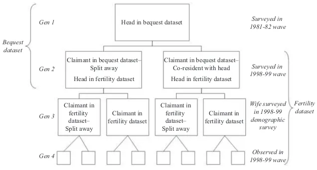
Using the 1998–99 wave of the REDS survey, I construct two data sets. The fi rst is a “bequest data set” that contains information on the bequests of land received by 1999 heads from their fathers upon the father’s death, and is used to test for strategic bequests in Section IV.A. The second is a “fertility data set” that contains information on the fertility choices made by the 1999 claimants when the head is still alive, and is used to test for strategic fertility in Section IV.B.
Figure 3 shows four generations of a joint family. The bequest data set contains the
fi rst generation as the head, and the second generation as claimants. In the fertility data set, the heads are the second generation, and the claimants are the third genera-tion. This confi guration allows me to test, using the same families, the implications on the previous generation’s bequest behavior on the subsequent generation’s fertility behavior.
IV. Empirical Analysis
The theoretical model of strategic bequests predicts a differential im-pact of bequest behavior on survival and health outcomes for girls compared to boys. Hence, the fi rst objective of the econometric exercise is to check whether, as suggested by Equation 5, a claimant’s share of the bequest is infl uenced positively by the number of sons compared to daughters. This establishes the relative value of sons to claim-ants in the bequest game.6 The second objective is to test strategic fertility behavior
predicted in Equations 12 and 14, that is, whether a claimant’s fertility in a joint family is infl uenced by the number of boys and girls that the other claimants have. To test this behavior, I propose a “within- family fertility” test that estimates the differential fertility response of claimants in a joint family to the other claimants’ boys and girls, a test comparing claimants’ behavior when they are in joint families versus indepen-dent families, and a test of claimants’ behavior in land- owning and non- land- owning households. In addition, I calculate the number of siblings born to girls and boys in joint families, and compare this to outcomes in stem families where there is no bequest game. Finally, I calculate the impact of strategic fertility on gender differences in child mortality in six states of India.
A. Strategic bequests
The bequest data set contains a cross- sectional snapshot of the family at the time of the head’s death. It consists of those land- owning families that were part of a single land- owning household in 1981–82, but had split into at least two households by 1998 following the head’s death in the interim.7 Using the demographic questionnaire, I construct a complete fertility history between waves and calculate the number of sons and daughters for each claimant at the time of the head’s death.
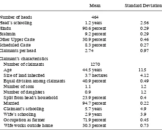
Table 1 contains summary statistics from the bequests data set. The bequest data set contains 1,270 claimants from 464 heads, with 2.74 claimants per head. Data on the head’s characteristics is sparse because all heads had died by the time of the
7. Note that the data set does not report intended bequest shares while the head is still alive, only the actual shares once he dies. This might create bias if heads’ preferences change systematically as they get older. How-ever, if the head’s primary objective is to preserve lineage or if future change in preferences is anticipated by claimants, then I expect this bias to be small.
Figure 3
1998–99 wave and were not directly surveyed. The average size of land inheritance is 3.7 hectares per claimant. Note that each claimant has, on average, 1.1 sons but only 0.9 daughters.
I check for evidence of strategic bequest behavior, where the share of a claim-ant’s inheritance (κij) is positively correlated with the number of sons (mij) that claim-ant i in family j has at the time of the head’s death, and negatively correlated with the sum of the other claimants’ sons ∑k≠imkj. Therefore, I specify the following model
(21) ij=␣0+␣1nij+␣2
k≠i
∑
nkj+␣3nij*rij+␣4rij* k≠i∑
nkj+␣5Xij+␣6Yj+ijwhere nij=[mijfij]′, ␣1=[␣1m␣1f], ␣2=[␣2m␣2f], ␣3=[␣3m␣3f], and ␣4=
[␣
4m␣4f]. To confi rm the strategic bequest hypothesis, I expect that ␣1m>0 and
␣2m<0 corresponding to the theoretical predictions in Equation 5. The coeffi cients on two interaction terms nij*r
ij and rij∗ ∑k≠inkj indicate the correlation between the Table 1
Summary Statistics of Bequest Data Set
Mean Standard Deviation
Number of heads 464
Head’s schooling 1.2 years 2.56
Hindu 90.6 percent 0.29
Brahmin 9.2 percent 0.29
Other Upper Caste 30.9 percent 0.46
Scheduled Caste 8.3 percent 0.27
Claimants per head 2.74 0.97
Claimant’s characteristics
Number of claimants 1270
Age 44.5 years 11.5
Size of land inherited 3.7 hectares 4.12
Equal division among claimants 40.9 percent 0.49
Number of sons 1.1 1.2
Number of daughters 0.9 1.2
Split from head’s household 23.9 percent 0.4
Married 94.7 percent 0.22
Claimant’s schooling 5.7 years 4.9
Wife’s schooling 2.9 years 3.9
Occupation as farmer 71.9 percent 0.45
Wife works outside home 30.3 percent 0.73
Source: REDS 1998–99, matched with REDS 1981.
number of sons and daughters for a claimant who has moved away from the head’s household.8
This specifi cation must be qualifi ed by controlling for the claimant’s residence choice rij and other observed claimant- specifi c factors Xij that might infl uence bequest preferences such as age at the time of inheritance and years of schooling for the claim-ant and his wife, which are importclaim-ant since a better- educated and technologically savvy claimant might have better access to reproductive technology (including sex- selective abortion). Also included are dummy variables that indicate whether or not the claimant is a farmer and if the claimant’s wife works outside the home as these might be potentially correlated with the bequest share. Yj includes family- specifi c factors such as the head’s education, occupation as farmer and other demographic character-istics. Finally, ij captures unobserved claimant- specifi c factors such as diligence at work or fi lial relationship with the head, and is assumed to be distributed i.i.d. normal with zero mean.
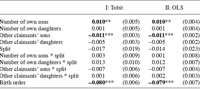
The results from Specifi cation 21, which tests for the association between family structure and received bequest shares, are presented in Table 2. Column I shows the results of a dual- censored tobit model, where the bequest shares are censored below 0 and above 1. Column II shows the results from an OLS regression. Both sets of estimates are close to each other, and show that an additional son is associated with a one percentage point increase in the claimant’s share of the land bequest. This mirrors the increase in bequest share for the other claimants when they have an additional son (1.1 percentage points). The opposite effects of relatively equal magnitude suggest that claimants with more sons receive more land, and that grandsons from different claimants are substitutes for each other.9
Note that a claimant’s residence away from the head’s household (while remaining in the same family) does not seem to impact his inheritance. The standard errors as-sociated with ␣3 and ␣4 are large and the coeffi cient cannot be statistically distin-guished from zero. Hence, it is unlikely that claimants make fertility and residence choices concurrently in order to receive a larger inheritance.
These results establish that the number of own and other claimants sons are impor-tant factors determining the bequest received by the claimant, and provide support to an important assumption made in the theoretical model that sons, not daughters, receive the dominant share of land bequests. Thus, claimants have an important incen-tive to maximize the number of sons they have if they live in a joint family where the head is still alive and owns land.
B. Strategic fertility
In the fertility data set, each observation consists of a man who is older than 15 years of age. Each adult man is counted as one among multiple claimants in a joint family
8. The effect of moving away is theoretically ambiguous because splitting from the head’s household might indicate that the claimant has been disinherited and is no longer a part of the bequest game or that the claim-ant is already in a strong position, irrespective of the number of sons, to receive a signifi cant share of the inheritance.
where the head is still alive, as the sole claimant in a stem family where the head is still alive, or else as the head of a nuclear family. In joint and stem families, the claimant can either be co- resident within the same household or part of a separate household while remaining in the same family.
The man’s wife answers questions on her fertility history, which allows me to create a retrospective panel data set. Schultz (1972) reports that recalled data on pre- and postnatal child mortality is more reliable closer to the survey period.10 Therefore, the sample is restricted to 1992–98, which leaves 43,612 claimant- family- year observa-tions in the panel from 5,090 families over seven years.
In most data sets, the potentially endogenous selection of claimants into classifi ca-tion as joint, stem, or independent (nuclear) families is a major concern. The long time period over which the REDS panel is observed, 1981–99, helps to alleviate some of these concerns. Claimants might live within the household occupied by the joint fam-ily head or set up a separate household. Consistent with observed bequest behavior, split off sons retain status as claimants in the joint family household headed by their father as long as the father is alive. Thus, in the data set used in this paper, coresidence
10. Recalled fertility data suffers from bias from two main sources (Schultz 1972). The primary reason is that events in the distant past are reported less frequently than events in the recent past. The secondary reason is that women who reside in the household in the distant past might be different from those who reside in the household in the recent past. Maternal mortality is a signifi cant factor in the high death rate among adult women in South Asia. Therefore, the mortality rate is higher among more fertile women, leading to nonran-dom sample selection if we survey only women who are alive in 1998–99.
Table 2
Strategic Bequest Results
I: Tobit II: OLS
Number of own sons 0.010** (0.005) 0.010** (0.004)
Number of own daughters 0.001 (0.005) 0.001 (0.004)
Other claimants’ sons –0.011*** (0.003) –0.011*** (0.002)
Other claimants’ daughters –0.005 (0.003) –0.005 (0.002)
Split –0.017 (0.019) –0.014 (0.023)
Number of own sons * split 0.003 (0.009) 0.001 (0.008)
Number of own daughters * split 0.013 (0.010) 0.012 (0.007)
Other claimants’ sons * split –0.007 (0.006) –0.007 (0.004)
Other claimants’ daughters * split 0.001 (0.006) 0.002 (0.003)
Birth order –0.080*** (0.006) –0.079*** (0.007)
Source: REDS 1998–99.
is not a condition for membership in a joint family. Coresidence is a characteristic of a claimant and accounted for using an indicator variable, r
i∈{0,1}, that represents the
claimant’s residence within or outside the head’s household respectively. This variable is assigned based on the circumstances of departure and household division as re-ported in the REDS data set. Sons who become household heads after their father’s death are categorized as independent heads whereas those who split before their fa-ther’s death are categorized as part of the joint family till the head dies. Unless a joint family head dies and distributes the bequest, a claimant who lives separately is not classifi ed as an independent (nuclear) family. Thus, the potentially endogenous selection of claimants into joint, stem, or independent families is accounted for in case of splits since 1981, which controls for most cases for the analysis in the period 1992–98.
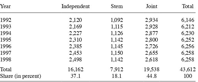
With this assignment, the fertility data set has 16,162 observations as nuclear fami-lies, 7,912 observations in stem famifami-lies, and 19,538 observations in joint families. Table 3 reports the number of claimants in each family type by year. The numbers change over time due to two reasons. First, the sample grows as new claimants attain 15 years of age. Second, the number of joint families decreases and the number of independent families increases as heads die and claimants form their own independent families as a result. I assume that both these events occur exogenously.
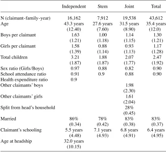
Table 4 reports the summary statistics for the fertility data set. Independent couples have on average more children (3.21) than claimants in joint families (2.07). This might refl ect the fact that independent heads are older, with average age 43.3 years, compared to claimants in stem (27.6 years) and joint families (31.5 years) and are therefore more likely to have completed their fertility. An important feature of joint families is the signifi cantly worse sex ratio. The ratio of girls to boys is 0.82 in joint families, 0.88 in stem families, and 0.97 in independent families. Thus, the data sug-gests that survival of girls is worse in joint families compared to other family types.
Table 3
Claimants in Fertility Data Set
Year Independent Stem Joint Total
1992 2,120 1,092 2,934 6,146
1993 2,169 1,115 2,928 6,212
1994 2,227 1,126 2,877 6,230
1995 2,310 1,142 2,800 6,252
1996 2,385 1,145 2,726 6,256
1997 2,453 1,150 2,655 6,258
1998 2,498 1,142 2,618 6,258
Total 16,162 7,912 19,538 43,612
Share (in percent) 37.1 18.1 44.8 100
Statistics for school attendance and health expenditures for independent and joint families corroborate the mortality statistics.11
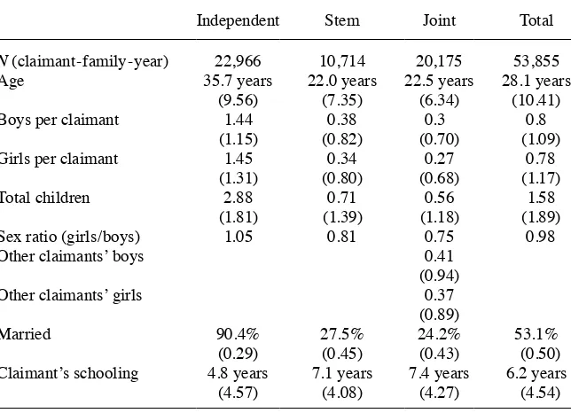
In order to alleviate the concern that these empirical patterns are specifi c to the REDS sample and not robust to a different draw of the data, I replicate the sum-mary statistics for claimants in the National Family Health Survey’s 1998 wave and present these in Table 5. Matching the distribution of respondents in REDS 1998, the smallest fraction of claimants live in stem families. However, because it is not
11. Differences in claimants’ schooling in Table 4 are consistent with younger couples as claimants in joint families, and relatively older couples as independent heads since formal education has expanded considerably in India over the past few decades (The PROBE Team 1999).
Table 4
Summary Statistics of Fertility Data Set
Independent Stem Joint Total
N (claimant- family- year) 16,162 7,912 19,538 43,612
Age 43.3 years 27.6 years 31.5 years 35.4 years
(12.40) (7.60) (8.90) (12.0)
Boys per claimant 1.63 1.00 1.14 1.30
(1.21) (1.18) (1.15) (1.21)
Girls per claimant 1.58 0.88 0.93 1.17
(1.39) (1.14) (1.13) (1.28)
Total children 3.21 1.88 2.07 2.47
(1.87) (1.87) (1.77) (1.92)
Sex ratio (Girls / Boys) 0.97 0.88 0.82 0.90
School attendance ratio 0.91 0.9 0.88 0.90
Health expenditure ratio 0.9
Other claimants’ boys 1.98
(2.30)
Other claimants’ girls 1.61
(2.04)
Split from head’s household 28%
(0.45)
Married 86% 78% 83% 83%
(0.34) (0.42) (0.38) (0.37)
Claimant’s schooling 5.5 years 7.1 years 6.8 years 6.4 years
(4.48) (4.93) (4.91) (4.95)
Age at headship 32.0 years
(10.15)
Source: REDS 1998–99
possible to identify split- off claimants from joint family households, the number of independent households compared to claimants in joint families is larger in NFHS (22,966 independent households compared to 20,175 claimants living in joint fami-lies). If the likelihood of splitting increases with age, the claimants who remain in stem and joint families are signifi cantly younger than those in independent families. I observe this in the NFHS data set as the average age of claimants in stem and joint families is 22.0 and 22.5 years, respectively. These relatively young ages imply that these claimants have not yet married or completed their fertility, and the number of children they have is small. However, the sex ratio corresponding to each fam-ily type matches REDS 1999. The fraction of girls to boys is 1.05 in independent families, very close to the natural rate, but only 0.81 in stem families and 0.75 in joint families. Other demographic characteristics also match REDS (1999) summary statistics.
1. Within- family fertility
In this section, I test whether the probability that a claimant in a joint family tries to have another child is positively impacted by the number of boys that the other
claim-Table 5
Summary Statistics of Fertility Data Set from NFHS
Independent Stem Joint Total
N (claimant- family- year) 22,966 10,714 20,175 53,855
Age 35.7 years 22.0 years 22.5 years 28.1 years
(9.56) (7.35) (6.34) (10.41)
Boys per claimant 1.44 0.38 0.3 0.8
(1.15) (0.82) (0.70) (1.09)
Girls per claimant 1.45 0.34 0.27 0.78
(1.31) (0.80) (0.68) (1.17)
Total children 2.88 0.71 0.56 1.58
(1.81) (1.39) (1.18) (1.89)
Sex ratio (girls / boys) 1.05 0.81 0.75 0.98
Other claimants’ boys 0.41
(0.94)
Other claimants’ girls 0.37
(0.89)
Married 90.4% 27.5% 24.2% 53.1%
(0.29) (0.45) (0.43) (0.50)
Claimant’s schooling 4.8 years 7.1 years 7.4 years 6.2 years
(4.57) (4.08) (4.27) (4.54)
Source: National Family Health Survey 1998–99
ants have, corresponding to the theoretical prediction in Equation 12.12 The other claimants’ daughters are not future heirs in the family lineage, and have a negative impact on the claimant’s own fertility (equation 14). Jointly, strategic fertility implies that the relative difference between the impact of the other claimants’ sons and daugh-ters is positive and signifi cant. To test for this proposition, I specify a model with a binary outcome ijt that is 1 if a claimant i in joint family j reports a pregnancy in year t, and 0 otherwise.
(22) ijt=0+1nijt+2
k≠i
∑
nkjt+3Xijt+4Vij+ familyjt+ yeart+εijtwhere ni=[mifi]′, 1=[1m1f], and 2=[2m2f]. In this model, the claimant reports a pregnancy based on the number of sons and daughters (nijt) he already has. I expect a negative relationship between the number of children and the probability that the claimant will try for one more, that is, 1m<0 and 1f <0. Because sons have value in the bequest game while daughters do not, Equation 11 predicts that 1m<1f. Strategic fertility is identifi ed by the components of 2. In particular, Equation 12, which implies 2m>0, and Equation 14, which implies 2f <0, combine to predict that 2m−2f >0.
One threat to this specifi cation is from omitted variables that might impact fertility. Therefore, I control for observable time- varying characteristics (Xijt) of the claimant and his partner that impact fertility, such as age and marital status as well as time- invariant characteristics (Vij) such as years of schooling and participation in the formal work force. Fertility decisions might be infl uenced by factors that are specifi c to the joint family rather than just the claimant. For example, the head or his wife might have unobservable preferences for grandchildren, and encourage the claimants to have more children. Controlling for these preferences is important to isolate the degree to which the claimants’ fertility is responding to the other claimants’ family structure, and not to unobserved preferences for grandsons that are correlated across claimants. To ac-count for this, I exploit the panel characteristics of the data set and include family fi xed effects, familyjt, that control for all observed and unobserved time- invariant character-istics that are common across all members of the joint family. Year fi xed effects ac-count for time- varying factors that impact fertility across all claimants and families, such as availability of food due to variations in nationwide monsoon rainfall (yeart). Finally, εijt is an i.i.d. term that represents unobserved factors that might impact fertility.
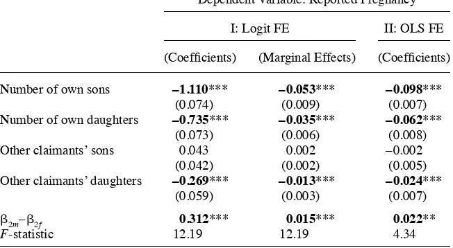
Column I of Table 6 presents the logit fi xed effects coeffi cients from estimating equation (22). The number of own sons and daughters has a large, negative, and statis-tically signifi cant impact on a claimant’s fertility. An additional son decreases fertility by 5.3 percent and an additional daughter reduces fertility by 3.5 percent. This is expected and confi rms that fertility decreases with additional children, and that ad-ditional sons cause greater decreases than daughters.
The marginal effect associated with an additional son for the other claimants is posi-tive (+0.2 percent), but the associated standard errors are large. The other claimants’
daughters have a large negative impact on the claimant’s fertility (–1.3 percent) that is statistically different from the null at the 1 percent level, a fi nding that is consistent with the theoretical prediction of Equation 14. The equality between 
2m and 2f is
strongly rejected with an F- statistic of 12.19. These empirical fi ndings are consistent with the theoretical prediction that claimants exhibit a differential fertility response to other claimants’ sons and daughters (Equation 15). The fi ndings also suggest that the major channel through which strategic fertility operates is a greater decrease in fertil-ity with additional daughters of the other claimants.13
Column II in Table 6 reports the results of the OLS fi xed effects model. The fi nd-ings of this model are consistent with those in Column I. The other claimants’ sons have a small, negative (–0.2 percent) and insignifi cant impact on fertility, whereas
13. To confi rm that the fertility response results from intrafamily differences in family structure and not from spurious correlations or unobserved factors, I conduct a falsifi cation exercise where claimants are randomly reassigned to different families in the data. The impact of these other claimants’ sons and daughters ought to be very close to zero and statistically indistinguishable from zero. I fi nd that the coeffi cients associated with the sons and daughters of the randomly assigned claimants is very small with large standard errors in both the fi xed and random effects versions of the model. Additionally, the equality of coeffi cients (2m=2f) is not rejected with an F- statistic of 0.03 in the fi xed effects model and 0.20 in the random effects model. Detailed results are available on request.
Table 6
Results of Test of Strategic Fertility Within Joint Families
Dependent Variable: Reported Pregnancy
I: Logit FE II: OLS FE
(Coeffi cients) (Marginal Effects) (Coeffi cients)
Number of own sons –1.110*** –0.053*** –0.098***
(0.074) (0.009) (0.007)
Number of own daughters –0.735*** –0.035*** –0.062***
(0.073) (0.006) (0.008)
Other claimants’ sons 0.043 0.002 –0.002
(0.042) (0.002) (0.005)
Other claimants’ daughters –0.269*** –0.013*** –0.024***
(0.059) (0.003) (0.007)
β2m–β2f 0.312*** 0.015*** 0.022**
F- statistic 12.19 12.19 4.34
Source: REDS 1998–99
the other claimants’ daughters have a negative and statistically signifi cant impact (–2.4 percent). The difference in the point estimates associated with the other claim-ants’ sons and daughter is, as expected, positive and signifi cant at the 5 percent level. Therefore, the results of this test are also consistent with the strategic fertility hypothesis.14
2. Joint versus independent families
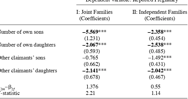
This test employs the death of the previous head during the period of our study as a natural experiment to observe fertility behavior within the same family.15 Accord-ing to Caldwell, Reddy, and Caldwell’s (1984) framework presented in Section I, a family with a living head plus multiple adult claimants constitutes a joint family, but the claimants form independent families once the head dies. Thus, assuming that the head’s death is not associated with fertility behavior, the death of the head, and the disbursement of the bequest offers a natural experiment to test for strategic fertility behavior within the same family. The theory predicts that strategic fertility ought to be salient only while the head is still alive and the claimants are living in joint families but not so once the head dies—at which point the bequest is distributed and the claim-ants form independent families. I test this proposition by estimating the specifi cation in Equation 22 for families where the head is alive and where the head has died, that is, claimants residing in a joint or independent family, respectively. As before, the specifi cation includes a term for claimant age, to control for the fact that claimants are older after the head dies than before.
Table 7 reports the results of this test. Truncating the sample reduces the number of observations to less than a tenth of the full sample. The coeffi cients under “I” represent the impact of family structure on claimants who are part of a joint family before the head’s death, and the coeffi cients under “II” represent the impact on the same claimants once they have formed independent households after the head’s death. The claimant’s own sons and daughters cause large declines in fertility both before and after the head’s death, although the effect is larger before than after. The most probable reason for this difference is that even controlling for age, higher order births are more likely after head’s death, and thus the marginal reduction in the probability of an ad-ditional pregnancy is greater. The fertility response to the other claimants’ family structure before the head’s death mirrors the results from the previous section where the coeffi cient associated with the other claimants’ sons is statistically indistinguish-able from the null (–0.765) but the coeffi cient associated with the other claimants’ daughters is large, negative, and signifi cant (–2.141, p < 0.01). However, once the head dies and the land is distributed among the claimants, both coeffi cients associated with other claimants’ sons and daughters are negative and statistically signifi cant (–1.492 and –2.042, respectively). Although the difference 2m–2f is larger in joint
14. Another potential concern is the claimant’s potentially endogenous choice of coresidence within the same household. To address this concern, I also estimate a bivariate probit model of joint fertility and residence choice. The results from this model are not qualitatively different from those in reported in Table 6, confi rm-ing that residence choice is not a signifi cant factor in the strategic fertility game. Detailed results are available from the author on request.
families compared to independent families, the relevant F- tests cannot reject the null in either case.
3. Land ownership
The fi nal analysis examines the heterogeneous impact of land ownership on strategic fertility. If the head owns no land that he can bequeath, then claimants might have diminished incentives to respond to each other’s family structure. To check for differ-ences on the basis of land ownership, I estimate the logit fi xed effects model (Equa-tion 22) separately for landless and land owning families.
Table 8 presents the results of the test of strategic fertility and land ownership. Column A represents claimants in joint families where the head does not own any land. Column B reports claimants in joint families with a land- owning head. The fi rst fi nd-ing is that while the claimant’s own family structure is a statistically signifi cant deter-minant of fertility, other claimants’ daughters have signifi cant effects in both family types while other claimants’ sons do not. The coeffi cient associated with an additional son for other claimants is positive in land- owning families (0.041) and negative in landless families (–0.527) but neither are statistically different from the null. At the same time, both the coeffi cients associated with the other claimants’ daughters are negative and statistically signifi cant (–0.238 for land- owning families and –1.614 for landless families, p < 0.01 for both). The difference 
2m–2f is statistically signifi cant Table 7
Strategic Fertility in Joint Versus Independent Families
Dependent Variable: Reported Pregnancy
I: Joint Families (Coeffi cients)
II: Independent Families (Coeffi cients)
Number of own sons –5.569*** –2.358***
(1.231) (0.454)
Number of own daughters –2.067*** –2.538***
(0.593) (0.485)
Other claimants’ sons –0.765 –1.492***
(0.662) (0.431)
Other claimants’ daughters –2.141*** –2.042***
(0.678) (0.467)
β2m–β2f 1.376 0.55
F- statistic 2.21 1.14
Source: REDS 1998–99
in both cases, at the 1 percent level for landowning families and at the 10 percent level for landless families. One potential explanation for this fi nding is that claimants in landless families might compete to receive other immovable assets (such as the house). Strategic fertility might also have become imbibed as a cultural trait among rural households. Examples of such behavior include the process of “Sanskritization” where lower castes adopt the practices and rituals of higher castes to move up the social hier-archy. Lower caste families, less likely to own land, might mimic the inheritance and fertility practices of landowning families, which might be a possible explanation for the fi ndings in this section.
C. Implications of strategic fertility
To show how strategic fertility behavior yields health and mortality differences in outcomes for boys and girls, I fi rst demonstrate that the average girl in the population lives in families with more children than the average boy. Thus, even without differ-ences in resource allocations by parents toward children of different gender, the aver-age girl will receive smaller share of resources than the averaver-age boy, explaining poorer outcomes. Let fij and mij represent the number of daughters and sons born to claimant i
in family j. The number of siblings for any one of that claimant’s children is sij. The number of siblings for the average girl and boy are s
f and sm, respectively. Table 8
Strategic Fertility in Land Owning and Landless Families
Dependent Variable: Reported Pregnancy
A: Landless Families (Coeffi cients)
B: Land- Owning Families (Coeffi cients)
Number of own sons –1.730*** –1.085***
(0.468) (0.081)
Number of own daughters –2.127*** –0.745***
(0.566) (0.080)
Other claimants’ sons –0.527 0.041
(0.438) (0.045)
Other claimants’ daughters –1.614*** –0.238***
(0.532) (0.063)
β2m–β2f 1.087* 0.280***
F- statistic 2.77 8.52
Source: REDS 1998–99
(23) s larger for joint families where strategic fertility is salient compared to stem families where it is not. Table 9 reports that the average girl has 0.280 excess siblings compared to the average boy in joint families, in contrast to 0.156 excess siblings for the average girl in stem families. The difference in the excess siblings between stem and joint families is driven by fewer siblings for the average boy in a joint family. s
f for stem
families (2.757) is close to sf for joint families (2.761). However, the difference in sm
for stem families (2.600) and s
m for joint families (2.481) is large.
16 This is consistent
with the theory presented in Section 0 that predicts that a joint family with many boys is more likely to observe declines in fertility compared to similar stem families or families with many girls in either family type.
Next, I use estimates from Arnold, Choe, and Roy (1998) to calculate the extent to which the differences in family structure are associated with greater mortality for girls in six major states of India.17 I estimate the marginal effect of the claimant’s existing sons and daughters and the other claimants’ sons (B) and count the number of observa-tions in each cell ( ⌬). I assume that the probability of a male birth is p = 1 / 2. Arnold, Choe, and Roy (1998) report the mortality rates for boys (⍀m) and girls (⍀f) given the claimant’s existing family structure. Thus, the excess female deaths from strate-gic fertility behavior are B×⌬×(1− p)⍀f −B×⌬× p⍀m. I also estimate the prob-ability of another pregnancy reported conditional only on the claimant’s sons and daughters ( ⌫). Therefore, the overall excess female deaths from having a child are
⌫×⌬×(1−p)⍀f −⌫×⌬× p⍀m. Thus, the fraction of excess female deaths in India due to strategic fertility behavior is
16. Excess siblings for the average girl is not a trivial outcome of a sex ratio skewed against girls. Even with a skewed sex ratio, random assignment of girls and boys to households will yield the same number of siblings for both the average girl and boy.
17. Arnold, Choe and Roy (1998) report mortality rates only for these states.
Table 9
(24) B×⌬×(1−p)⍀f −B×⌬× p⍀m
⌫×⌬×
(
1− p)
⍀f −⌫×⌬× p⍀mTable 10 reports the fraction of excess female deaths explained by strategic fertility behavior for six states. The greatest impact of strategic fertility is in the Green Revo-lution states of Punjab, Haryana, and Rajasthan where the value of land (Figure 1) is greatest, and agriculture yields the largest share of income (Figure 2). Four percent of the female shortage in Punjab, and 7 percent of the shortage in Haryana and Rajasthan is explained by my model. In Orissa, where agricultural yields are low, strategic fertil-ity tied to bequests of agricultural land is not a large incentive for fertilfertil-ity behavior. In Kerala, where matrilineal descent is practiced among many communities, 39 percent of the shortage of boys is explained by fertility induced by land bequest motives. These back of the envelope calculations also predict a small shortage of boys in Tamil Nadu, which is inconsistent with Census data. One possible explanation for this mis-match is that the fertility rates are calculated for the period 1992–98, whereas the source for the sex ratio is the 2001 Census.
V. Strategic Fertility and Land Inheritance Laws in India
The theoretical model described in the earlier sections assumes that heads and claimants have the ability to make bequest and fertility choices without binding legal constraints. The interpretation of the empirical results in subsequent sec-tions also assumes that legal constraints are not signifi cant. Therefore, to ensure that the theoretical model is credible and empirical results are robust, I analyze the inheri-tance laws in India and their potential impact on bequests and fertility in greater detail. For Hindu families that comprise the vast majority of households in India, inheritance
Table 10
Differential Mortality Due to Strategic Fertility
Excess Female Deaths
Fraction of Excess
State
Number of Observations
Strategic
Fertility All Reasons
Female Deaths Explained
Observed Sex Ratio (Census)
Haryana 304 0.021 0.286 7% 861
Rajasthan 471 0.025 0.376 7% 922
Punjab 491 0.010 0.285 4% 874
Orissa 232 0.002 0.161 1% 972
Tamil Nadu 127 –0.003 –0.026 –11% 986
Kerala 186 –0.003 –0.008 –39% 1058