Directory UMM :Data Elmu:jurnal:M:Mathematical Social Sciences:Vol38.Issue3.Nov1999:

Assessing dependence among subjects’ responses

*

Francesca Cristante , Egidio Robusto

Department of General Psychology, University of Padova, Via Venezia 8, 35131 Padova, Italy Accepted 1 June 1998

Abstract

The aim of this study consists in the definition of a particular subject parameter, whose purpose is to test the dependence among subjects’ responses where the subjects are a couple or a group. In this context a model is proposed. The Response Dependence of Subjects Model (RDSM) treats couples or well-defined small groups as units characterized by two parameters, a location parameter and a dispersion parameter which is a measure of the dependence among subjects’ responses within each group. The binomial function provides a frame of reference for interpreting the dependence parameter. An application of the RDSM with dyadic data is presented.  1999 Elsevier Science B.V. All rights reserved.

1. Introduction

There are many situations in psychology for which theory and data analysis at dyadic or small group levels, rather than the individual level, is appropriate. Social, de-velopmental and clinical psychologists, for instance, talk about relationship in the couple, referring to interactive, cooperative, competitive couples, etc. (Griffin and Gonzalez, 1983). In particular for social psychologists, a major problem is not only analysis of the relationships within a small group or couple, but also obtaining data which reflect the small group or couple as a unit. Deal (1995) points out that the unit of analysis has been a critical problem in the study of well-defined groups, and specifically the family, for many years.

The aim of this study consists in the definition of a particular subject parameter, whose purpose is to test the dependence among subjects’ responses, where the subjects are a couple or a group, henceforth referred to as a ‘subgroup’. Response dependence is expected since operations involved in the members’ responses may be characterized by

*Corresponding author. Tel.:139-49-8276-686; fax:139-49-8276-600. E-mail address: cristant@psico.unipd.it (F. Cristante)

dependence, interpreted as a sort of implication of one another’s responses. In other words, if the persons are two, for instance, and one person gives a positive answer to a question, his / her answer might imply a positive answer of the other person also. However implication does not mean always equal answers, it might also be that a positive answer of one person implies tendentially a negative answer of the other person. According to this perspective, responses of members of well-defined subgroups of persons which belong to a larger group are likely to be dependent, even if independence of the responses of the members of the larger group is previously demonstrated. That is, independence of persons’ responses might fail if such persons are analyzed within well-defined subgroups. The model presented here – called Response Dependence of Subjects Model (RDSM) – belongs to the family of the Rasch models (Fisher and Molenaar, 1995). It is inscribed in the context of the properties of the Rating Formulation for ordered response categories by Andrich (1978), sharing the same algebraic form.

Before proceeding to the presentation of the RDSM, some principal aspects of the Rating Formulation Model and the Binomial Model are reviewed in the next section.

2. The rating formulation model and the binomial model

2.1. The Rating Formulation Model

According to Andrich (1985) the general rating model can be derived by making the following assumptions and definitions:

• in a Likert-type questionnaire the rating mechanism is based on a continuum with

m11 successive categories separated by thresholdstc, c51,2, . . . , m; • at each threshold a separate dichotomous response is given;

• the Simple Logistic Model by Rasch is applied at each thresholdtc, giving

expf2t 1c ysb 2 ddg

]]]]]]

P Yh c5yub,d,t 5cj _g , (1)

whereg is a normalizing factor; Y is a Bernoulli random variable at the threshold cc

that takes the value y51 if the threshold is exceeded and y50 otherwise; b2d

corresponds to the combination of the person parameterb and the item parameterd; the parametersb andd represent the locations of the person and the item respectively on the latent trait;

m

• from the set of all 2 possible outcomes the acceptable response patterns are restricted to the m11 patterns forming a Guttman (Guttman, 1954) structure, that is (0, 0, . . . , 0), (1, 0, . . . , 0), (1, 1, . . . , 0), . . . , (1, 1, . . . , 1), where each indicates the successive thresholds exceeded;

exceeded), 2 for the third category (first and second thresholds exceeded), and so on until the last category for which it takes the value m.

On the bases of the above definitions the Rating Formulation Model takes the form

exp cf x1xsb 2 ddg ]]]]]]

P Xh 5xub,d, c, mj5 _g (2)

x

where cx5 2oc51 tc, with c05cm5 0, x51,2, . . . , m.

The c category coefficients are expressed in terms of the m thresholds_x t₁,t₂, . . . ,t_m

on the continuum.

m

From the definition of c and c , it follows thatx m oc51 ct 50 for all thresholds. In the case that the thresholds are equidistanttx112t 5t 2 tx x x215l*.0. With this assump-tion, the coefficients c take the following simple structurex

1

]

cx5₂x ms 2xdl*5x ms 2xdl

wherel*52l giving the model

exp x mf s 2xdl 1xsb 2 ddg

]]]]]]]]

P Xh 5xub,d,l, mj5 _g (3)

x

That cx5x ms 2xdl 5 2oc51 ct can be easily demonstrated with any value of m. For instance, consider m54 in which case there are 5 ordered categories. Then from

cx5x ms 2xdl, c050, c153l, c254l, c353l and c450. Further, since cx5 2

x

oc51 ct 5 2 t 1s 1 ...1txd, cx5cx212tx, so thatt 5x cx212c . Then, for mx 54,t 5 21

3l,t 5 2 l2 ,t 5 l3 ,t 54 3l, in which case the successive distances between thresholds are, as required, given byt 2 t 5 t 2 t 5 t 2 t 52 1 3 2 4 3 2l.

2.2. The Binomial Model

The general form of the Binomial Model is

m x m2x

P Xh 5xup, mj5

s d

_x p s12pd (4)

where 0 and m are the minimum and maximum values for X andp is the parameter of the probability distribution. Defining the probability parameter p by

expsb 2 dd

]]]]]

p 5 (5)

11expsb 2 dd

and entering (5) into (4) transform the model into the form

x m2x

expsb 2 dd expsb 2 dd

m _{]]]]] ]]]]]}

P Xh 5xub,d, mj5

s d

_x

F

G F

12

G

11expsb 2 dd 11expsb 2 dd

m

x _{exp ln}

f s d

_1xs_{b 2 d}d

g

expsb 2 dd

m_{]]]]]] ]]]]]]]}x

5

s d

_x m5 m (6)

11exp b 2 d 11expb 2 d

[image:4.612.54.422.104.159.2]

Table 1

Category coefficients and threshold values for m52, m53 and m54

Variable X m52 m53 m54

0 1 2 0 1 2 3 0 1 2 3 4

m

ln

s d

_x 5cx 0 0.69 0 0 1.10 1.10 0 0 1.39 1.79 1.39 0 t 5x cx212cx 20.69 0.69 21.10 0 1.10 21.39 20.41 0.41 1.39

where b 2d corresponds to the combination of the person parameter b and the item parameterd; m corresponds to the number of response categories of an item.

A characteristic of the Binomial Model is that it is formed from dichotomous Bernoulli responses satisfying independence and having the same probability parameter

p. These properties permit the model to provide a frame of reference for interpreting dependence.

2.3. The dependence parameter l

m

If cx5ln

s d

_x , the Rating Formulation Model of Eq. (2) is equal to the Binomial Model

m

of Eq. (6). Thus, being cx5ln

s d

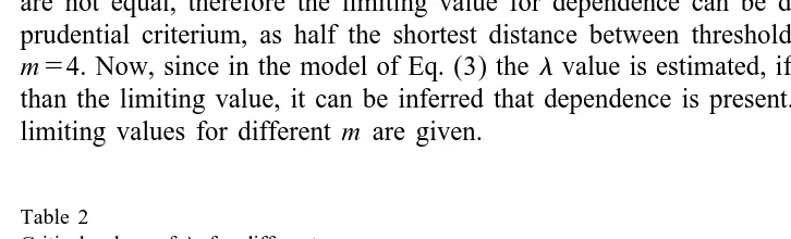
_x in the Rating Formulation Model, then the response categories of an item can be interpreted as being equivalent to those formed from independent Bernoulli responses with the same probability parameter. On the other hand, as shown in Andrich (1985), if the estimates of the thresholds are closer together than values that correspond to the binomial coefficients, then the responses can be considered dependent. Table 1 shows the values of the thresholds for binomial coefficients for

m52, m53 and m54. For m52 and m53 the thresholds are equidistant. In these cases half the distance between thresholds can be considered the limiting value for depen-dence, they are 0.69 and 0.55 respectively. For m$4 the distances between thresholds are not equal, therefore the limiting value for dependence can be defined, adopting a prudential criterium, as half the shortest distance between thresholds, that is 0.41 for

m54. Now, since in the model of Eq. (3) thelvalue is estimated, if such value is less than the limiting value, it can be inferred that dependence is present. In Table 2 thel_l

limiting values for different m are given.

Table 2

Critical values ofll for different m

m ll

[image:4.612.59.422.509.619.2]

As Andrich (1985, 1982) points out, it is most interesting to notice that the coefficient

cx5x ms 2xd of the parameter l is quadratic and symmetric, thus l is scored quadratically by a function of successive integers. In this way, the parameterlcan also be considered as an index of dispersion of the responses. An other important feature ofl

is that although it is defined initially bytx112t 5x 2l .0, it is possible to interpret both a value of zero and a negative value forl. Aslis a coefficient of a quadratic function, it characterizes the curvature of the exponent of Eq. (3) and therefore also the curvature of the distribution of this equation. If l.0 the distribution is unimodal, if l50 the distribution is uniform and if l ,0 the distribution is U-shaped.

2.4. Estimation procedure

A method presented by Andrich et al. (1982) is considered here. The person parameter is conditioned out so that the item parameterdand the dependence parameter

l are estimated simultaneously, but independently of the unknown person parameterb. The person parameter is then estimated unconditionally taking as known the estimate of parametersdandl. The estimation procedure involves considering items in pairs and is a generalization of a method for dichotomous items (Andrich, 1988). The set of simple

N

sufficient statistics is s5ov51x for the item location parameter, where the summation is N

over N persons, v is any person and x50, 1, . . . , m; t5ov51 x ms 2x for the itemd k

dependence parameter, where the summation is also over N persons; and r5oi51x for

the person location parameter, where the summation is over k items and i is any item. The values s and t are the jointly sufficient statistics for parameters d and l

respectively.

2.5. Goodness of fit

As far as goodness of fit is concerned for item and person parameters d and b, the item–person interaction procedure is taken into consideration (Andrich, 1988). Given the model of Eq. (4) and the estimates of the parametersd, b andl, in this procedure the probability of any outcome is predicted by inserting these values in the equation. Tests of fit for specific persons and items are then obtained by summing and transforming standardized residuals across items and persons respectively.

3. Response dependence of subjects model (RDSM)

[image:6.612.156.319.88.244.2]

Fig. 1. Matrix subjects by items.

In the figure, Xvi50 if subject v does not choose item i; Xvi51 if subject v chooses item i.

The k items describe a dimension according to an increasing order of intensity. The local independence of the items is assumed from results of previous Rasch analyses, in which responses of all persons were also independent.

The N subjects of the matrix of Fig. 1 are subdivided in h groups of n persons each. Each subgroup represents a well-defined unit which can take values X50, 1, . . . , n. The matrix becomes like that of Fig. 2.

In the figure, each group has n subjects and n can vary in size; Xgi50 if no subject in the subgroup chooses item i; Xgi51 if one subject in the subgroup chooses item i;

[image:6.612.156.319.453.607.2]

Xgi52 if two subjects in the subgroup choose item i and so on, until Xgi5n if n subjects

in the subgroup choose item i.

The RDSM takes the form of Eq. (7)

exp x n

f s

_g2x

d

l 1_g x

s

b 2 d_{g i}

dg

]]]]]]]]]

P X

h

gi5xubg,di,lg, ng

j

5 _g (7)

g

where Xgi5x is the score of subgroup g on item i; n is the number of persons ing

subgroup g; bg is the location parameter of subgroup g on a dimension; di is the location parameter of item i on the same dimension. The local independence of the k items has already been accepted from previous studies; lg is the dependence parameter of subgroup g; gg is the normalizing factor.

The analogy of Eq. (7) with Eq. (3) is evident. In order to appreciate the way the RDSM accounts for dependence among responses of persons who form a group, the parameterlg has to be taken into special consideration. By comparing the estimatedlg

with the limiting value of Table 2 it is possible to check whether the independence condition is violated or not. Thelg value is designed to absorb the dependence among the n individuals that form a subgroup belonging to a larger subgroup of N persons for which the independence property has already been tested. That is to say, the in-dependence among persons might be violated if tested within well-defined subgroups of similar individuals.

3.1. Equality of subjects’ responses

The second question is concerned with the equality (or at least closeness) of the probability that the n persons, who belong to a subgroup, have of responding. In order to reply to this question the answers of the n persons, who respond to k items, are considered as replications of the same dichotomous event, which means equal probabili-ty of choosing an item. In order to assess if the n persons have an equal probabiliprobabili-ty of responding, a Chi-square statistic can be applied on a contingency table where the number of items endorsed by each person is compared with the other persons’ choices. Testing the hypothesis of equi-probability of endorsing an item does not violate the relative independence of the persons who belong to the same group, in relation to a

1

wider group.

1

The Chi-square is applied to a univariate contingency table where the variable is ‘person’ and the levels of the variable are the n persons. The null hypothesis is H : p0 i5p , for some 00 ,p0,1, for all i51, . . . , n. To give an example, let us consider n53 persons and k items, and let us suppose that one person endorses l items out of k, the second endorses q items and the third u items. The observed number of items that are endorsed is then l1q1u and the expected number of items for each person is ls 1q1u / 3. The Chi-square statisticd will test if the three persons have equal probability of responding, comparing the number of items that they endorse. In other words, rejecting H means that the probability of responding to k items for each person is0

4. The interaction of the two binomial conditions ‘independence by equal probability’

In terms of the manifestation of the binomial properties in the persons’ responses, in Table 3 different cases are considered in order to describe the interaction between such properties. Some illustrative numerical examples will be made for n52.

Case 1 – Independence-Equal probability. Both the binomial conditions are satisfied.

As it appears in cell (1) of Table 3,l 5 lg l, that is to say there is no implication among responses of persons who belong to a subgroup and there is also similarity among responses. For n52 persons and a 232 table where both persons have probability 0.50 to endorse an item, the joint probabilities of the entries (0, 0), (0, 1) or (1, 0) and (1, 1) are 0.25, 0.50 and 0.25, when the binomial conditions are satisfied.

Case 2 – Independence-Unequal probability. Only one of the binomial conditions is

satisfied. The heterogeneity of the response probabilities generate a response distribution which is more peaked than the binomial and, as it appears in cell (5) of Table 3,l . lg l. If the case is n52 and for instance person 1 and person 2 have probabilities 0.10 and 0.90 to endorse an item respectively, the joint probabilities in the 232 table are 0.09, 0.82 and 0.09. The probability distribution is more peaked than the binomial.

When there is independence among responses, the cases in cells (2) and (6) of Table 3 are not admissible; the cells are structurally empty.

Case 3 – Dependence-Equal probability. Only one of the binomial conditions is

satisfied. Independence is violated. As it appears in cells (3) and (4) of Table 3, the l

parameter is affected by the sign of the covariation. For n52, when both person 1 and person 2 have probability 0.50 to endorse an item, if the joint probabilities are 0.20, 0.60 and 0.20, the covariation is negative, l . lg l and the probability distribution is more peaked than the binomial. However if the covariation is positive and the joint probability values are, for instance, 0.30, 0.40 and 0.30, l , lg l and the probability distribution is flatter than the binomial.

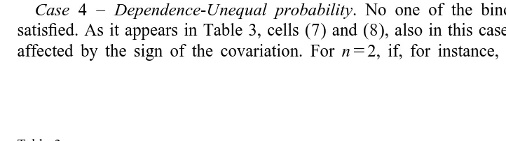
Case 4 – Dependence-Unequal probability. No one of the binomial conditions is

[image:8.612.56.417.518.619.2]

satisfied. As it appears in Table 3, cells (7) and (8), also in this case thelparameter is affected by the sign of the covariation. For n52, if, for instance, the probabilities of

Table 3

Interaction of independence by probability Independence

No violation Violation

Negative Positive Negative Positive covariation covariation covariation covariation

Probability Equal (1) (2) (3) (4)

l 5 lg l – l . lg l lg ,ll

Unequal (5) (6) (7) (8)

endorsing an item are 0.60 and 0.40 and the joint probabilities are 0.20, 0.40, 0.20 and 0.20 respectively for the entries (0, 0), (0, 1), (1, 0) and (1, 1) in a 232 table, the covariation is negative, l . lg land the probability distribution is more peaked than the binomial. However if the probabilities are 0.30, 0.30, 0.10 and 0.30, the covariation is positive, lg ,ll and the probability distribution is flatter than the binomial.

On the base of the previous considerations and examples, it is to notice that whenl_g ,ll (cells (4) and (8) in Table 3) there is no doubt about violation of independence among subjects’ responses; whereas when l . lg l (cells (3), (5) and (7) in Table 3) three different interpretations are possible. In order to decide about dependence or independence among responses when l . lg l, inspection of the sign of the covariation and of the equal probability property are needed. If equal probability and negative covariation coexist, there is dependence among responses, but if unequal probability and negative covariation interact in the data (cells (5) and (7) in Table 3) it might be either a case of dependence or a case of independence. In this situation a hypothesis of independence could be made on the base of the level of inequality of the probabilities of the persons’ responses. The more heterogeneous the probability among responses is, the more likely it is that the responses are independent. If n52 and if for instance person 1 has probability 0.10 and person 2 has probability 0.90 to endorse an item, there is a strong tendency to independence which could be easily illustrated by means of the joint probabilities in a 232 table.

5. Estimation procedures of bg and lg parameters

For estimating both thebgandlg parameters, the procedure suggested by Andrich et al. (1982) to estimate the parameters of Eq. (3) is adopted here for the parameters of Eq. (7). Such a procedure is an extension of the method for dichotomous data described by Andrich (1996). The procedure, already mentioned in a previous paragraph, when adapted to the particular purposes of model (7), consists in conditioning out the item parameter di so that the two subgroup parameters bg and lg are estimated simul-taneously, but independently, of the item parameter. The method used involves considering subgroups in pairs.

For any two subgroups g and q ( g ± _{q) of the matrix of Fig. 2 and for a particular}

item i, the Eq. (8) is given

P X , X

hs

gi qi

d

udi,bg,lg, n ,g bq,lq, nq

j

exp x n

f s

_{g g}2x_g

d

l 2_g x_{g i}d 1x n_q

s

_q2x_q

d

l 2_q x_qb 1_q

s

x_g1x_q

d g

d_i ]]]]]]]]]]]]]]]]]

5 (8)

g ggi qi

where X , X

s

gi qi

d

represents the ordered pair of responses Xgi of subgroup g and Xqi of subgroup q to item i;ggi andgqi are normalizing factors.

P X , X

hs

g q

d

ubg,lg, n ,g bq,lq, n , sq 5xg1xq

j

exp x n

f s

_{g g}2x_g

d

l 2_g x_gb 1_g x n_q

s

_q2x_q

d

l 2_q x_qb_q

g

]]]]]]]]]]]]]]]]]

5 U (9)

O

exp c n

f s

g2c

d

l 2g cb 1g ss2c nd

s

q2s1c

d

l 2q ss2cdbq

g

c5L

where L5max 0, s

s

2nq

d

and U5min s, n .

s

g

d

The item parameterdi drops out of expression (7). Considering all possible scores s

[

s

0,m_g1m_q

d

and all possible subgroup pairs, it follows that the likelihood functionL

is given by Eq. (10)

h

exp

F

sh21d

O

s

tgl 2g rgbg

d

G

g51

]]]]]]]]]

L 5 h h ng1nq U ks_gq (10)

P P P O

S D

egqcs

q.g

g51 s50 x5L

k k

where tg5oi51x ngi

s

g2x ; rgi

d

g5oi51x ; k is the number of items; h is the number ofgi s

subgroups; kgq denotes the number of items which received a total score of s from subgroups g and q; egqcs5exp c n

f s

g2c

d

l 2g cb 1g ss2c nd

s

q2s1c

d

l 2q ss2cdbq

g

.

The next step consists in the maximization of the log likelihood function by setting the first derivatives of this function with respect to lg and bg equal to zero. The equations obtained, both for lg andbg, are solved using a modified Newton-Raphson algorithm. The derivation of the two equations for the parameters of Eq. (4) is an application of the method presented in Andrich et al. (1982). The item parameterdi is then estimated unconditionally taking as known the estimated parametersbgandlg. The RUMM v. 2.7 computer program by Andrich et al. (1996) is suggested for the estimation of the parameters.

6. Test of fit procedures

The test of fit for the subgroup location parameterbg is based on the item-subgroup interaction residuals. The procedure employed involves the prediction of the scores (0, 1, . . . , n) for each subgroup in each item, given the model of Eq. (7) and the parameter estimates. Tests of fit for specific subgroups are obtained by summing and transforming standardized residuals across items.

With the estimated parameters bg, lg and di, the probability of any outcome is obtained by Eq. (7). Then the expectation value and the variance of the score of subgroup g on item i are given by the usual expressions

n

E X

s

gi5x

d

5

O

xP ,xgi x50

n

where Pxgi5P X

s

gi5x is the probability obtained with Eq. (7) and V X

d

s

gi5x

d

5

s

ox50

2 n 2

x2E X

f

s dg

gi

]]]]

zgi5 ]] .

V X

s d

gi

œ

This residual has a mean of 0 and a variance of 1.

The sum of the statistic zgi across either persons or items is equal to zero. Therefore, considering in this context the test of fit for the parameterbg, the sum of the squares of the residuals across k items is used to derive the fit statistic:

2 2

zg5

O

zgi k

with expected value

2 2 2

E z

s d

g 5E

S D

O

zgi 5

O

E z

s d

gi

k k

and variance

2 2 2

V z

s d

g 5V

S D

O

zgi 5

O

V z

s d

gi

k k

.

2

A standardized residual is calculated for z by Eq. (11)g

2 2

z 2E z

f

g

s dg

g

]]]]

S15 ]]₂ (11)

V z

s d

g

œ

2 2

Since zg$0, the minimum value S is1 2E z , while its maximum is in principle

s d

g 1`; this makes the distribution asymmetrical. A transformation that makes the distribution more symmetrical is the ratio of Eq. (12)

2 2 2

E z

s df

g ln zg2ln E z

s dg

g

]]]]]]

S25 ]]₂ (12)

V z

s d

g

œ

the S ratio is symmetrical around 0 and has a mean of 0 and a variance of 1. The shape2

of the distribution approximates the standard normal distribution.

7. An illustrative application: stress and resources of handicapped children’s parents

subscales, named ‘Family problems’ (QRS ), ‘Pessimism’ (QRS ) and ‘Child’s1 2

problems’ (QRS ), where each subscale contains 24 items. In the validation process with3

the Italian subjects, Rasch analyses were carried out for each subscale; the fit to the model was satisfactory for all items. For illustrative purposes, only the results concerning the QRS subscale are shown and discussed in this context.1

The QRS items were applied to 44 couples, that is 88 parents of children affected by1

asthma or thalassemia. The responses of the 88 subjects, analyzed in previous studies, showed local independence on the base of Rasch analyses. The number of subjects is rather small, nonetheless it should be noted that this case is concerned with measuring and studying the effects of small subgroups (couples) of people in the context where the items, as mentioned above, have already been checked and validated for the required properties.

The subjects were from different Italian regions both in the north and south of the country and belonged to the middle class social level; their age ranged from 31 to 64; the age of their pathologic children ranged from 6 to 25. The following main questions were posed: (a) what positions do the 44 parent couples occupy on the QRS1

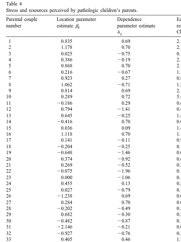
dimension?; (b) are the responses of the partners of each couple statistically independent or dependent?; (c) how similar are the responses of the parents in each couple? In order to estimate the positions of the couples on the dimension and to assess the dependence / independence of the responses, Eq. (7) was applied. Whereas the equi-probability of the responses was tested by means of a Chi-square; due to the small frequencies a continuity correction was used. In Table 4 the parent couple identification number and the location parameter estimatebgon the QRS dimension are shown. The1 lgdependence parameter and the Chi-square statistic are also presented. The fit to the model of the couples’ responses was elaborated with Eq. (12) and the Chi-square statistic was obtained as explained in Footnote 1. The location estimatebg describes the level of stress and the family resources as perceived by the couple. A low estimated value describes inadequate resources and a consequent high level of stress, on the contrary a high estimated value corresponds to adequate resources and, as a consequence, a low level of stress.

In Table 4, it can be noted, for instance, that parent couple number 44 perceives satisfactory resources in the family and manifests a low level of stress, since b 5₄₄

1.599. On the contrary, couple number 31 perceives inadequate resources and expresses a high level of stress since b 5 231 2.146.

The fit to the model is satisfactory except for couple 15 (S251.75, obtained by means of Eq. (12), p50.04), denoting an anomalous response pattern to the 24 items which are indicators of the QRS dimension.1

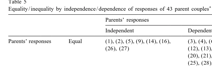
The interpretation of the parameterlgin terms of independence / dependence between parents’ responses must take into consideration also the equality / inequality of the responses within each couple. An analysis of the difference between parents’ responses was carried out by means of the Chi-square statistic and the statistical significance of the difference was checked ( p,0.05). In Table 5 the interaction between independence / dependence and equality / inequality is shown; in the four cells the 43 couples (couple 15 have been excluded in these results) are distributed considering the limiting value

[image:13.612.56.419.129.614.2]

Table 4

Stress and resources perceived by pathologic children’s parents.

Parental couple Location parameter Dependence Equi-probability of number estimatebg parameter estimate responding

lg Chi-square

1 0.835 0.69 2.13

2 1.178 0.70 2.13

3 0.025 20.75 0.18

4 0.386 20.19 2.13

5 0.868 0.70 2.13

6 0.216 20.67 1.11

7 0.923 0.27 0.83

8 1.062 20.71 1.25

9 0.814 0.69 2.13

10 0.289 0.72 5.42*

11 20.186 0.29 0.67

12 0.794 21.41 0.40

13 0.645 20.25 1.43

14 20.416 0.70 0.06

15 0.036 0.09 1.42

16 1.118 0.70 1.11

17 0.141 20.11 0.91

18 20.204 20.25 0.13

19 20.648 21.46 0.06

20 0.374 20.92 0.63

21 0.269 20.52 0.22

22 20.075 21.96 0.18

23 0.000 21.06 0.10

24 0.455 0.13 0.22

25 0.027 20.79 0.18

26 21.238 0.69 0.04

27 0.284 0.70 0.08

28 20.202 20.49 0.36

29 0.682 20.30 0.29

30 20.482 20.87 0.12

31 22.146 20.21 0.05

32 20.927 20.76 0.21

33 0.405 0.46 1.70

34 21.235 0.17 0.07

35 21.446 0.23 0.34

36 20.648 21.46 0.06

37 20.345 0.48 0.12

38 20.139 22.10 0.18

39 21.219 0.09 0.96

40 0.011 22.02 0.18

41 20.740 0.49 0.48

42 20.953 20.79 0.04

43 0.686 20.79 0.83

44 1.599 20.90 0.67

[image:14.612.54.419.103.219.2]

Table 5

a

Equality / inequality by independence / dependence of responses of 43 parent couples Parents’ responses

Independent Dependent

Parents’ responses Equal (1), (2), (5), (9), (14), (16), (3), (4), (6), (7), (8), (11), (26), (27) (12), (13), (17), (18), (19), (20), (21), (22), (23), (24), (25), (28), (29) (30), (31), (32), (33), (34), (35), (36), (37), (38), (39), (40), (41), (42), (43), (44)

Unequal (10)

a

The numbers in the cells correspond to the identification couple numbers of Table 4.

Data in Table 5 point out the following main results: (a) the parents, who on the base of Rasch analyses all showed a good fit to the model, when analyzed in couples, show that independence – one of the fundamental properties of the Rasch models – is violated in 79% of couples. That is, when analyzed individually the 86 subjects respond independently, whereas when considered in couples they are no longer independent in most cases. Only 9 out of the 43 couples give independent answers to the items. (b) As expected, the majority of couples, 34 out of 43, give dependent and similar (equal) responses to the items characteristic of the QRS dimension. In other words, the two1

parents not only express similar opinions in relation to their family resources and stress, but the father’s opinion implies the mother’s and vice versa. Such an implication might be interpreted as a sort of reciprocal conditioning of the two parents. (c) Both the binomial properties, independence and equal probability, are not violated in the responses of eight couples; that is, these parents give similar responses, but there is no implication and no reciprocal conditioning. (d) Only the members of couple 10 give different responses and moreover do not influence each other when answering. For this couple the probability of endorsing an item is 0.09 for person 1 and 0.42 for person 2. A hypothesis of independence can be made.

8. Summary and final remarks

any other small social group). Dependence is expected since, due to the fact that people who belong to a group share similar experiences, they might influence one another. Another problem is also posed: do people who belong to a small group also give equal or similar answers? An interaction between dependence and equal answers is expected, although equal responses are not necessarily associated to dependent responses. The following are all conceivable situations: the case of persons not influencing one another when expressing an attitude or opinion and giving independently very similar answers, or those who give both independent and different answers, or those who show implications when expressing an attitude or opinion and nonetheless give different answers.

The proposed model is a Rasch model and is an interpretation of the Rating Formulation for ordered response categories by Andrich (1978). It is specified by three parameters: two location parameters for item and group of persons and one dependence parameter. This last parameter allows assessment of whether the members of a couple or group give independent answers to questionnaire items or not. Independence is defined by the binomial coefficient, which means that a hypothesis of stochastic independence of the subjects’ responses is made. If independence is rejected, dependence is interpreted as a sort of conditioning of one another’s responses. In order to interpret the dependence parameter according to the binomial conditions – independence and equal probability – the probability of equal responses is also taken into consideration. It is argued that the persons who belong to a group and who respond to an item can be considered as replications of the same dichotomous event, that is, they have equal probability of choosing a specific item. In order to assess the equality of the probability, a Chi-square statistic is applied on a contingency table where the number of items endorsed by each person belonging to a subgroup is compared with the other persons’ choices. If the equi-probability hypothesis is rejected, then the persons have unequal probability of responding to the items. The interaction of the two binomial conditions generates four cases which assume different interpretations from a psychological point of view:(a) dependent and equal responses (the main hypothesis); (b) dependent and unequal responses; (c) independent and equal responses (binomial conditions); (d) independent and unequal responses.

members of any subgroup for whom there are good reasons to believe that they are linked because of common experiences, might show dependence when expressing attitudes, feelings or opinions. As far as interpretation is concerned, in this study dependence among subjects’ responses was considered as an implication and / or conditioning of one another when expressing attitudes, opinions or feelings. This interpretation of dependence does not exclude that there might be groups characterized by dependence and unequal responses, in the sense that conditioning of one another might produce different and some time even opposite reactions in the people and as a consequence different attitudes or behaviors. More analyses and theoretical discussion should be made on this point in order to achieve a better insight and formulate a more articulate interpretation of the violation of independence and the violation of equality among responses of subjects who belong to well-defined small groups.

References

Andrich, D., 1978. A rating formulation for ordered response categories. Psychometrika 43, 561–573. Andrich, D., 1982. An extension of the Rasch model for ratings providing both location and dispersion

parameters. Psychometrika 47, 105–113.

Andrich, D., 1985. A latent-trait model for items with response dependencies: implications for test construction and analysis. In: Embretson, S.E. (Ed.), Test Design, Academic Press, Orlando, pp. 245–275.

Andrich, D., 1988. Rasch Models for Measurement, Sage, Beverly Hill.

Andrich, D., De’Ath, G., Lyne, H., Hill, P., Jennings, J., 1982. Disloc: A Program for Analysing a Rasch Model with Two Item Parameters, State Education Department, Western Australia.

Andrich, D., Luo, G., Sheridan, B., 1996. RUMM-Rasch Unidimensional Measurement Models. User’s guide, 1996. (Available from David Andrich, Murdoch University, Murdoch, Western Australia 6150). Deal, J.E., 1995. Utilizing data from multiple family members: a within-family approach. Journal of Marriage

and the Family 57, 1109–1121.

Fisher, G., Molenaar, I.W. (Eds.), 1995. Rasch Models. Foundations, Recent Developments and Applications, Springer-Verlag, New York.

Friedrich, W.N., Greenberg, M.T., Crnik, K., 1983. A short form of the questionnaire on resources and stress. American Journal of Mental Deficiency 88 (1), 41–88.

Griffin, D., Gonzalez, R., 1983. Correlational analysis of dyad-level data in the exchangeable case. Psychological Bulletin 118 (3), 430–439.

Guttman, L., 1954. The principle components of scalable attitudes. In: Lazarsfeld, P.F. (Ed.), Mathematical Thinking in the Social Sciences, The Free Press, Glencoe, IL, pp. 216–257.