Vol. 44 No. 1 2014 83–118
REALIZED NON-LINEAR STOCHASTIC VOLATILITY
MODELS WITH ASYMMETRIC EFFECTS AND
GENERALIZED STUDENT’S
T
-DISTRIBUTIONS
Didit Budi Nugroho* and Takayuki Morimoto**
This study proposes a class of realized non-linear stochastic volatility models with asymmetric effects and generalized Student’st-error distributions by applying three families of power transformation—exponential, modulus, and Yeo-Johnson—to lagged log volatility. The proposed class encompasses a raw version of the realized stochastic volatility model. In the Markov chain Monte Carlo algorithm, an effi-cient Hamiltonian Monte Carlo (HMC) method is developed to update the latent log volatility and transformation parameter, whereas the other parameters that could not be sampled directly are updated by an efficient Riemann manifold HMC method. Empirical studies on daily returns and four realized volatility estimators of the Tokyo Stock Price Index (TOPIX) over 4-year and 8-year periods demonstrate statistical evidence supporting the incorporation of skew distribution into the error density in the returns and the use of power transformations of lagged log volatility.
Key words and phrases: Hamiltonian Monte Carlo, non-linear stochastic volatility, realized variance, skew distribution, TOPIX.
1. Introduction
Volatility modelling of asset returns is one of the most prolific topics in the financial econometrics time series literature, including the autoregressive condi-tional heteroskedasticity (ARCH) model proposed by Engle (1982), the general-ized ARCH model (GARCH) by Bollerslev (1986), the stochastic volatility (SV) model proposed by Taylor (1982) and Kim et al. (1998), and the realized vari-ance (RV) approach introduced by Andersenet al.(2001). Theoretically, the SV model is much more flexible, realistic, and better performing than the ARCH-type models (Ghyselset al.(1996)) and generalized ARCH (GARCH)-type mod-els (Kimet al.(1998), Carneroet al.(2001), Yu (2002)) since an innovation term is embedded in the volatility dynamics.
Recently, models joining returns and realized measures have been developed via a measurement equation that relates the conditional variance of the returns to the realized measure, which also includes ‘asymmetry’ to shocks for making a very flexible and rich representation. Koopman and Scharth (2013) provide a short overview of the joint models outside the SV methodology. In particular, Hansen et al. (2011) introduced the Realized GARCH model that substantially
Received February 12,2014. Revised May 21,2014. Accepted June 25,2014.
*Department of Mathematics,Satya Wacana Christian University,Jl. Diponegoro 52-60,Salatiga, Central Java 50711,Indonesia. Email: [email protected]
improves the empirical fit compared to the standard GARCH models that only use return series. In the context of the SV model, very closely related studies of joint models have been proposed by Takahashiet al.(2009), Dobrev and Szerszen (2010), and Koopman and Scharth (2013). Their model is known as the realized stochastic volatility (RSV) model.
This study focuses on Takahashiet al.’s (2009) version. Recently, Takahashi et al.(2014) extended their model by applying a general non-linear bias correction in the RV measure and the generalized hyperbolic skew Student’s t-distribution (SKT distribution), which includes normal and Student’s t-distributions as spe-cial cases. The models studied by Takahashi et al. (2009) and Takahashi et al. (2014) have already incorporated the asymmetric volatility phenomenon, which captures the negative correlation between current return and future volatility. We label Takahashi et al.’s (2014) asymmetric version of the so called RSVC model as the R-ASV model and then formulate this model as
which the autocorrelations are removed, exp(ht) characterizes the unobservable
variance of returns,Ytdenotes the log RV,ξ0is a linear bias correction parameter representing the effect of microstructure noise (ifξ0 >0) or that of non-trading hours (if ξ0 < 0), ξ1 is a non-linear bias correction parameter representing the persistence (correlation) of RV, α and φ represent the drift and persistence of log volatilities ht, respectively, and ρ captures the correlation between current
returns and future volatility. Jacquier and Miller (2010) and Takahashi et al. (2014) found that, in the presence of microstructure noise, the posterior mean of ξ1 deviates from the assumption of Takahashi et al. (2009) that ξ1 = 1 for the different realized estimators.
Tsio-tas (2009) instead of the linear version as in Takahashi et al. (2014). We refer to this extension of the R-ASV framework as therealized non-linear asymmetric stochastic volatility (R-NASV) model. The empirical results from Tsiotas (2009) provide evidence that the nonlinear version is a better fit than the linear version in the SV context. This study does not only investigate the use of exponen-tial and Yeo-Johnson transformations (as in Tsiotas (2009)) but also the use of modulus transformations for transformation of lagged volatility in Model (1.1). These transformations are indexed by the parameterλand were selected on the basis of the fact that these families permit transformed data to be non-positive and contain aλvalue that does not correspond to transformation (linear version) because the main idea is to transform log volatilityht. Notice that in the case of
the Yeo-Johnson transformation (Yeo and Johnson (2000)), interpretation of the transformation parameter is difficult as it has a different function for negative and non-negative values of transformed data. However, this family can be useful in procedures for selecting a transformation for linearity or normality (Weisberg (2014)).
Second, we apply two Hamiltonian Monte Carlo (HMC)-based methods within the Markov chain Monte Carlo (MCMC) algorithm to update the pa-rameters that cannot be sampled directly. Our MCMC simulation employs a Hamiltonian Monte Carlo (HMC) algorithm for updating the log volatility and transformation parameter. To update the other parameters that cannot be sampled directly, the implementation is to sample these parameters using the Riemann manifold HMC (RMHMC) algorithm proposed by Girolami and Calderhead (2011). In contrast to previous studies that have proposed the single-move or multi-single-move Metropolis-Hastings algorithm to estimate the SV model, in-cluding Tsiotas (2009), Takahashiet al.(2009, 2014), we propose the HMC-based methods since these methods update the entire log volatility at once. The HMC method has been shown to be more appropriate than the single move Metropolis-Hastings algorithm when sampling from high-dimensional, strongly correlated target densities (e.g., Takaishi (2009), Neal (2011), Girolami and Calderhead (2011)). Moreover, Girolami and Calderhead (2011) demonstrated that, among various sampling methods (including HMC), RMHMC sampling yields the best performance for parameters and latent volatilities, in terms of time-normalized effective sample size.
Regarding the parameters of the generalized Student’s t-distribution and power transformations, the data provide some evidence supporting the NCT distribu-tion and the non-linear volatility specificadistribu-tions. Thereafter, the performance of the new model is compared with those of competing new and old RSV models us-ing a modified harmonic mean method proposed by Gelfand and Dey (1994). We find that our empirical test presents significant evidence against the linear RSV model introduced by Takahashiet al.(2009) and Takahashiet al.(2014) and par-ticularly favors an SKT distribution. In addition, to address concerns about the sensitivity of MCMC output to prior choices, we show considerable robustness for priors of power parameterλwith very diffused distributional behavior.
This study is organized as follows. Section 2 introduces the four RV ap-proaches, existing leveraged RSV models, and new specifications of RSV models. In Section 3, we develop the HMC and RMHMC algorithms to estimate the parameters and latent variables of the proposed model. Section 4 discusses the computation of the marginal likelihood. The empirical results are presented in Section 5, and in Section 6, we present our conclusions and suggestions for ex-tending this study.
2. Volatility models 2.1. RV measures
At present, RV has become the benchmark volatility measure of intra-day high-frequency data (IHFD). RV is a non-parametric measure proposed by An-dersenet al. (2001) as a proxy for non-observable integrated volatility. Various versions of the RV measure, incorporating many improvements and modifica-tions, have been proposed previously. These include the bipower variation (BV, Barndorff-Nielsen and Shephard (2004)), the two-scales realized volatility (TSRV, Zhang et al. (2005)), and the realized kernel (Barndorff-Nielsen et al. (2008)). In this study, we compute the IHFD-based volatility measures using data sam-pled at four different frequencies: RV 1-min, RV 5-min, skip-one BV, and TSRV 5-min.
Suppose that a process occurring in day t is observed on a full grid {0 ≤ τt,0 ≤τt,1 ≤ · · · ≤τt,m}and pt,j denotes the log price on thejth observation grid
in dayt. Thejth percentage intra-day return is then defined as follows: Rt,j = 100×(pt,j−pt,j−1).
The basic daily RV is defined as the summation of the corresponding high-frequency intra-daily squared returns:
RVt= m
j=1 R2t,j.
Assuming the absence of jumps and microstructure noise and on the basis of quadratic variation theory, Andersenet al.(2001) showed that RVtconverges to
To extract the jump component from RV, Barndorff-Nielsen and Shephard (2004) proposed an empirical estimator called bipower variation (BV) that is defined as the sum of the product of adjacent absolute high-frequency intra-daily returns:
BVt=
π 2
m
j=2
|Rt,j||Rt,j−1|.
This approach is known to be robust in the presence of jumps in prices. Andersen et al.(2005) proposed a modification of the BV estimator and called it “staggered BV”. Assuming that microstructure noise is absent, these staggered BV mea-sures converge to the integrated conditional variance as observation frequency increases. In this study, we use the staggered (skip-one) BV defined by
BVt=
π 2 ·
1− 2
m
−1 m
j=3
|Rt,j||Rt,j−2|,
where the normalization factor in front of the sum reflects the loss of two obser-vations due to the staggering.
To control independent microstructure noise, Zhang et al.(2005) suggested a TSRV estimator based on sub-sampling, averaging, and bias-correction. This estimator is the bias-adjusted average of lower frequency realized volatilities com-puted onK non-overlapping observation sub-grids
TSRVt=
1 K
K
j=1
RV(tj),(avg)−m−K+ 1 K RV
(all)
t ,
which combines the two time scales (all) and (avg). The natural way to select the jth sub-grid, j = 1, . . . , K, is to start at τt,j−1 and subsequently observe everyKth sample point.
2.2. RSV models with asymmetric effect and generalized t-distribu-tion
In the SV models, Harvey and Shephard (1996), Jacquier et al.(2004), and Yu (2005) found strong evidence supporting the asymmetrical hypothesis of stock returns, which is a negative correlation between the errors of conditional returns and conditional log-squared volatility. Takahashi et al. (2009) confirmed that the asymmetry is also crucial in the RSV model. As explained by Yu (2005), if we assume corr(ǫt, vt+1) = ρ = 0 as in Harvey and Shephard (1996) instead of assuming corr(ǫt, vt) = ρ in Jacquier et al. (2004), the SV model becomes a
martingale difference sequence, by which asymmetry can be interpreted. According to previous studies, it is convenient to write
vt+1 =ρǫt+
1−ρ2η
t+1, for t= 1,2, . . . , T −1,
Areparameterization of the model yields
Furthermore, many empirical studies have shown that asset returns are char-acterized by heavy tails (excess kurtosis) that cannot be captured by the normal distribution. Geweke (1993), Watanabe and Asai (2001), and Jacquier et al. (2004) found that the Student’s t-distribution can capture the heavy-tailedness of the conditional distribution of daily returns. However, as the return distri-bution may exhibit skewness, a skewed version of the Student’s t-distribution might be more adequate in some cases. Several skew Student’s t-distributions have been previously proposed; for a short overview see Aas and Haff (2006). To accommodate flexible skewness and heavy-tailedness in the conditional distri-bution of returns, Barndorff-Nielsen (1977) proposed the generalized hyperbolic (GH) distribution that may be represented as anormal variance-mean mixture, which is given by
Tµ,β,a,b,c=µ+βZ +
√
ZV, (2.1)
where V ∼ N(0,1) and Z ∼ GIG(a, b, c) are independent and GIG represents the generalised inverse Gaussian distribution.
Aspecial case of the GH distribution is the SKT distribution that is simple, flexible, and easily incorporated into the SV model based on a Bayesian esti-mation scheme using the MCMC algorithm (Nakajima and Omori (2012)). The SKT distribution is obtained by assuminga=−12ν and c= 0, whereν denotes degrees of freedom (Aas and Haff (2006)). Following Nakajima and Omori (2012), we then assumeb=√ν, which yieldsZν ∼ IG(ν/2, ν/2), whereIG denotes the
inverse gamma distribution, and set µ = −βµν, where µz = E(Zν) = ν−ν2 and
ν >4. These yield the SKT distribution formulated as
Tν,β =β(Zν −µz) +
ZνV.
Its density is given as (Aas and Haff (2006)) f(x) = 2
whereKj is the modified Bessel function of the third kind of order j.
Using the SKT distribution, we propose a R-ASV model with SKT-errors distribution, called the R-ASV-SKT model, that takes the following form:
where zt ∼ IG(ν2,ν2) and (ζt, ut, ηt+1) ∼ N(0, I3). This model is an extension of the so called SVSKt model introduced by Nakajima and Omori (2012) for asymmetric SV models with SKT distribution that do not incorporate an RV equation. Incorporating an RV equation, the model is an extension of the so called ASV-RVC model introduced by Takahashi et al. (2009) for the asymmet-ric RSV model with normal distribution and ξ1 = 1. Takahashi et al. (2014) considered a similar approach to the above model with a standardized SKT dis-tribution the so called RSVCskt model. When β = 0, the above model reduces to the model with the central Student’s t-distribution (R-ASV-T model).
An alternative distribution to accommodate flexible skewness and heavy-tailedness in the conditional distribution of returns is the NCT distribution pro-posed by Johnson et al. (1995). If V and Qν are (statistically) independent
standard normal and chi-square random variables, respectively, the latter withν degrees of freedom, then
Tν,µ = µ+V
Qν/ν
= (µ+V)Zν,
where Zν ∼ IG(ν/2, ν/2), is said to have an NCT distribution with ν degrees
of freedom and non-centrality parameterµ. The probability density function of Tν,µ is
whereI(x|ν, µ) is the incomplete beta function with parameters ν and µ. Replacing a normal random variable ǫt in Model (1.1) with an NCT
distri-bution yields a new R-ASV model called the R-ASV-NCT model, which takes the following form:
This model is an extension of the so called ASV-nct model introduced by Tsiotas (2012) for the asymmetric SV model with NCT distribution that do not incor-porate an RV equation. When µ = 0, the R-ASV-NCT model reduces to the R-ASV-T model with the same degrees of freedom.
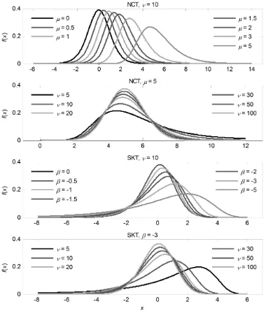
Figure 1. The NCT and SKT densities proposed,respectively,in equations (2.4) and (2.2) generated by combinations of parameters.
2.3. Power transformations
In statistics, data transformation is the usual method applied so that the data more closely satisfy the theoretical assumptions made in an analysis. Since Box and Cox (1964) published their seminal paper on power transformations, a number of modifications of the Box-Cox (BC) transformations have been pro-posed, both for theoretical work and practical applications. Because the purpose of this study is to transform log volatility ht, we select transformation families
from Manly (1976), John and Draper (1980), and Yeo and Johnson (2000) that consider any value in the real line and include a linear case.
Manly (1976) introduced a family of exponential transformations (ET) which is claimed to be quite effective at turning skewed unimodal distributions into nearly symmetric normal-like distributions taking the form:
PET(x, λ) =
John and Draper (1980) proposed the so-called modulus transformation (MT), which is effective for normalizing a distribution already possessing approximate symmetry about some central point, and it takes the form:
PMT(x, λ) = Johnson (2000) proposed a family of power transformations:
PYJ(x, λ) =
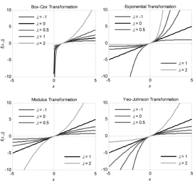
which is appropriate for reducing skewness toward normality and has many good properties of the BC power transformation family for positive variables. Thus, if the Box and Cox, Manly, and Yeo-Johnson transformations are used to make skew distributions more symmetrical and normal, the transformation family proposed by John-Draper can be used to eliminate any residual (positive) kurtosis. Figure 2 shows these transformations for the values ofλ=−1, 0, 0.5, 1, and 2.
Applying the above transformations families in the lagged state of the log volatility process in the R-ASV model, we propose an R-NASV model formulated as in equation (1.1) but the log volatility process now takes the form:
Figure 2. Characteristics of power transformation families.
where Pt =P(ht, λ) represents a family of power transformations. This model
is a non-linear extension of the ASV-RVC and RSVCskt models proposed by Takahashiet al. (2009, 2014), respectively, for the asymmetric RSV model with linear volatility process. Removing RV equation and asymmetric effects, the R-NASV model reduces to the so called nl-SV model proposed by Tsiotas (2009) for basic SV model with non-linear volatility process. We then call ETASV, R-MTASV, and R-YJASV for an R-NASV model corresponding to the exponential, modulus, and Yeo-Johnson transformations, respectively. In addition, the values of λET= 0, λMT= 1, and λYJ= 1 correspond to no transformation.
3. MCMC algorithm for R-NASV models
3.1. HMC and RMHMC methods
The HMC method alternately combines Gibbs updates with Metropolis up-dates and avoids the random walk behavior. This method proposes a new state by computing a trajectory obeying Hamiltonian dynamics (Neal (2011)). The trajectory is guided by a first-order gradient of the log of the posterior by apply-ing time discretization in the Hamiltonian dynamics. This gradient information encourages the HMC trajectories in the direction of high probabilities, resulting in a high-acceptance rate and ensuring that the accepted draws are not highly correlated (Marwala (2012)).
Let us consider position variables θ∈RD with densityL(θ|y)π(θ), where L(θ | y) is the likelihood function of given data y and π(θ) is our prior den-sity, and introduce an independent auxiliary variable ω ∈ RD with density p(ω) =N(ω |0,M). In a physical analogy, the negative logarithm of the joint probability density for the variables of interest, −L(θ) ≡ −ln(L(θ | y)π(θ)), denotes a potential energy function, the auxiliary variable ω is analogous to a momentum variable, and the covariance matrix M denotes a mass matrix. For standard HMC, the mass matrix is set to the identity.
The Hamiltonian dynamics system is described by a function of two variables known as the Hamiltonian function, H(θ, ω), which is a sum of the potential energyU(θ) and kinetic energyK(ω) (Neal (2011)),
H(θ, ω) =U(θ) +K(ω),
where U(θ) = −L(θ) +12log{(2π)D|M|} and K(ω) = 12ω′M−1ω. The second term on the right hand side in the potential energy equation results from the normalization factor. The deterministic proposal for the position variable is obtained by solving the Hamiltonian equations for the momentum and position variables, respectively, given by
dθ dτ =
∂H ∂ω =M
−1ω and dω
dτ =− ∂H
∂θ =∇θL(θ).
These equations determine howθandω change over a fictitious timeτ. Starting with the current state (θ, ω), the proposed state (θ∗, ω∗) is then accepted as the next state in the Markov chain with probability
P(θ, ω;θ∗, ω∗) = min{1,exp{−H(θ∗, ω∗) +H(θ, ω)}}.
Recently, Girolami and Calderhead (2011) proposed a new HMC method, the “RMHMC”, for improving the convergence and mixing of the chain. In their study, the covariance matrixM depends on the variableθand can be any positive definite matrix. M(θ) is chosen to be the metric tensor, i.e.,
M(θ) = cov
∂
∂θL(θ)
=−Ey|θ
∂2 ∂θ2L(θ)
and position variables, respectively, are now defined by dθ
dτ = ∂H
∂ω =M(θ)
−1ω
and
dω dτ =−
∂H
∂θ =∇θL(θ)− 1 2tr
M(θ)−1∂M(θ) ∂θ
+1 2ω
′M(θ)−1∂M(θ) ∂θ M(θ)
−1ω.
The above position variable equation requires calculation of the second- and third-order derivatives of L. This adds to the computational complexity of the algorithm, making it infeasible in many applications.
In practice, the differential equations of Hamiltonian dynamics are often simulated in a finite number of steps using the leapfrog scheme. Neal (2011) showed that the leapfrog scheme yields better results than the standard and modified Euler’s method. To ensure that the leapfrog algorithm is performing well, the step size and number of leapfrog steps must be tuned, which can usually be achieved with some experimentation. The “generalized leapfrog algorithm” operates as follows (for a chosen step size ∆τ and simulation lengthNL):
(i) update the momentum variable in the first half step using the equation
ωτ+(1/2)∆τ =ωτ−
1 2∆τ
∂H(θτ, ωτ+(1/2)∆τ)
∂θ ,
(ii) update the parameter θover a full time step using the equation
θτ+∆τ =θτ+
∆τ
2
∂H(θτ, ωτ+(1/2)∆τ)
∂ω +
∂H(θτ+ ∆τ, ωτ+(1/2)∆τ)
∂ω ,
and
(iii) update the momentum variable in the second half step using the equation
ωτ+∆τ =ωτ+(1/2)∆τ −
1 2∆τ
∂H(θτ+∆τ, ωτ+(1/2)∆τ)
∂θ .
The full algorithm for the HMC or RMHMC methods can be summarized in the following three steps (for covariance matrixM).
(1) Randomly draw a sample momentum vectorω∼ N(ω|0,M).
(2) Starting with the current state (θ, ω), run the leapfrog algorithm for NL
steps with step size ∆τ to generate the proposal (θ∗, ω∗). At every leapfrog
step, especially for the RMHMC algorithm, the values of ωτ+(1/2)∆τ and
θτ+∆τ are determined numerically by a fixed-point iteration method.
(3) Accept (θ∗, ω∗) with probability P(θ, ω;θ∗, ω∗), otherwise retain (θ, ω) as
3.2. MCMC simulation in the R-NASV models
Consider two observation vectorsR={Ri}Ti=1 and Y ={Yi}Ti=1, two latent variable vectors h ={hi}Ti=1 and z = {zi}Ti=1, and the parameter vectors θ1 = (ξ0, ξ1, σy), θ2 = (λ, α, φ, ϕ, ψ), and θ3 = (κ, ν), where κ is either µ or β. The
analysis presented here aims to obtain the estimates and other inferences of the proposed model parameters. Using Bayes’ theorem, the joint posterior density of the parameters and latent unobservable variables conditional on the observations is given as
By convention, we assume the following priors for the unknown structural pa-rameters:
whereBandGrepresent the beta and gamma densities, respectively. This choice of priors ensures that all parameters have the right support; in particular, the beta prior for φ would produce −1 < φ <1 that ensures stationary conditions for the volatility process.
3.2.1. Updating parameters (θ1, α, ϕ, ψ, κ)
are true values. We implement the MCMC scheme by first simulating random draws that can be sampled directly from their conditional posteriors:
−ψϕ2
In the following, we study ways to update the other parameters and latent variables that are unable to be sampled directly.
3.2.2. Updating parameter λ
On the basis of the joint density (3.1), the logarithm of the full conditional posterior density of λis represented by
L(λ)∝ − 1
which is not of standard form, and therefore we cannot sample from it directly. The RMHMC sampling scheme is not applicable to sampleλbecause the metric tensor required to implement the RMHMC sampling scheme cannot be explicitly derived from the above density. Therefore, we use the HMC algorithm for esti-mating the power parameterλ. This, specially in the leapfrog algorithm, requires evaluation of only the first partial derivative of the log posterior with respect to λ:
3.2.3. Updating parameter φ
An inspection of the joint density reveals that the logarithm of the full con-ditional posterior ofφ, which is given by
L(φ) ∝ 1
and is in non-standard form; thus, so it is not straightforward to sampleφ from this posterior. To sampleφ, we must be able to employ the RMHMC algorithm, and it is necessary to implement the transformation φ = tanh( ˆφ) for dealing with the constraint−1< φ < 1 so that it is restricted to the stationary region. The important aspect is that the leapfrog algorithm requires evaluations of the gradient vector and metric tensor of the log posterior. The partial derivative of the above log posterior with respect to ˆφis as follows:
Then, the metric tensor and its partial derivative, respectively, are 3.2.4. Updating parameter ν
The RMHMC algorithm is applicable to sample ν. Evaluations of gradient vector and metric tensor of the log posterior required in the leapfrog algorithm are as follows. The log posterior ofν is given by
L(ν) ∝ 1
0, for R-NASV-NCT model;
1
and the required gradient is given by
∇νL(ν) =
0, for R-NASV-NCT model;
−(ν2β
We then obtain the metric tensor M(ν) and its partial derivative with respect toν, respectively, as
where Ψ′(x) is a trigamma function defined by Ψ′(x) = dΨ(x)/dx, and Ψ′′(x)
0, for R-NASV-NCT model;
4β2
,for R-NASV-SKT model.
3.2.5. Updating the latent variable z
The logarithm of the full conditional posterior density of the latent variable z is
From this conditional density, draws can be obtained using the RMHMC algo-rithm and implementing the transformation zt = exp(ˆzt) to ensure constrained
sampling for zt>0. The gradient vector and metric tensor of the log posterior
required in the leapfrog algorithm are then evaluated as follows. The first partial derivative of the log posterior with respect to ˆzt is as follows:
∇ztˆL(zt) =−
whereI is an indicator function and
∂R˜t
t ,for R-NASV-NCT model;
−βzt1/2− 1
2R˜t, for R-NASV-SKT model.
Furthermore, the metric tensorM(z) is a diagonal matrix whose diagonal entries are given by
t<T, for R-NASV-NCT model;
β2ν Since the above metric tensor is not a function of the latent variable z, the associated partial derivatives with respect to the transformed latent variable are zero.
3.2.6. Updating the log volatilities h
Obviously, the posterior density of the latent volatility ht is in the
of only the first partial derivative of the log posterior with respect to ht. The
logarithm of the full conditional posterior ofh is expressed as
L(h) ∝ −1
and its partial derivatives with respect tohthave the following expressions:
∇h1L(h) =∇h1LR+∇h1LY −
4. Marginal likelihood and Bayes factors
The fundamental quantity in the Bayesian model comparison is the marginal density of the observed data (also known as the integrated likelihood or evidence ormarginal likelihood). Ahigher marginal likelihood for a given model indicates a better fit of the data by that model. For certain types of posterior simula-tors, several approximating methods for estimating the marginal likelihood from the MCMC output have been proposed, including Geweke’s estimator for impor-tance sampling, Chib’s estimator for Gibbs sampling, Chib-Jeliazkov’s estimator for the Metropolis-Hastings algorithm, and Meng-Wong’s estimator for a gen-eral theoretical perspective (Geweke and Whiteman (2006)). Another estimator, which is simpler, faster, and general, was proposed by Gelfand and Dey (1994).
In our model framework, the marginal likelihood of the Gelfand-Dey’s (GD) method is given by
where X is the matrix of the data, H is the matrix of the latent variables, f(·) can be any probability density function with the domain contained in the posterior probability density Θ, and p(θ,H) is the prior density for (θ,H) with respect to the Lebesgue measure. For computational convenience, we set f(θ,H) = f(θ)f(H), where f(H) = π(H) because the latent volatility H is high-dimensional. Then the marginal likelihood can be estimated by
ˆ
As explained by Geweke (1999), if f(θ) is thin tailed relative to the likeli-hood function, then f(θ)/L(X | θ,H) is bounded above and the estimator is consistent. Therefore, following Geweke’s (1999) suggestion, we choose f(θ) as a thin tailed truncated normal distributionN(θ∗,Σ∗), whereθ∗ and Σ∗ are the
posterior mean and covariance matrix of the θ draws, respectively. The domain of the truncated normal, Θ, is then constructed as
Θ ={θ: (θ(j)−θ∗)′(Σ∗)−1(θ(j)−θ∗)≤χ2.99(D)},
where D is the dimension of the parameter vector and χ2.99(D) is the 99th per-centile of the chi-squared distribution with D degrees of freedom. According to Θ, the normalizing constant of f(θ) is 1/.99 (Koopet al. (2007)).
Next, the prior densityπ(θ(j)) can be directly evaluated andL(X |θ(j),H(j)) is calculated by substitutingθ(j) and H(j) into the likelihood function. The log likelihood function of our model can be expressed as
L(R,Y |θ,h,z) = −Tln(2π)−1
model M1 with respect to the null model M0, we consider the ratio of their marginal likelihoods:
BF10=
mGD(X | M1) mGD(X | M0) .
On the basis of their similarity to the likelihood ratio statistic, general guidelines for the interpretation of Bayes factors were suggested by Kass and Raftery (1995). When the log Bayes factor is greater than 1 and less than 3, the null model is positively favored; when the log Bayes factor is greater than 3 and less than 5, the null model is strongly favored; and when the log Bayes factor is greater than 5, the null model is very strongly favored.
5. Empirical results on real data sets
This section applies the R-NASV models and the MCMC algorithm discussed in the previous section using TOPIX data over 4-year and 8-year periods. The data consist of intra-day high frequency observations from January 5, 2004 to December 30, 2011, excluding weekends and holidays.
5.1. Data in the evaluation period
The TOPIX data analysed in this study were divided into two periods: from January 2004 to December 2007 (984 trading days) and from January 2004 to December 2011 (1962 trading days). The asset price data were sampled at a frequency of 1 min when the market was open. Thetth percentage continuously compounded daily returnsRtis calculated as the difference between the logarithm
of the tth day’s closing pricePtand the logarithm of the (t−1)th day’s closing
pricePt−1, which is
Rt= 100×[ln(Pt)−ln(Pt−1)].
For extending the sampled volatility to a full-day volatility measure, Hansen and Lunde (2005) defined
RVHLt =c·RV(open)t , c=
%T
t=1(Rt−R)¯
%T
t=1RV(open)t
,
as a measure of the volatility on day t. We apply this adjustment to the four classes of RV, which are denoted as RV1HL for a 1-min sub-sampled RV, RV5HL for a 5-min sub-sampled RV, BV1HL for a skip-one BV, and TSRV5HL for a 5-min sub-sampled TSRV.
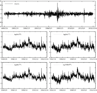
Figure 3. Time series plots of percentage daily returns and RVs of the TOPIX data from January 2004 to December 2011.
of the returns for both series is significantly greater than 3, indicating that the returns distribution is peaked relative to the normal (leptokurtic). Therefore, we fit the generalized Student’s t-distributions to the error distribution in our model.
5.2. MCMC setup and efficiency ofsimulators
Table 1. Descriptive statistics of daily returns and the logarithm of realized volatilities in the TOPIX data sets.
Period Data Mean SD Skewness Kurtosis JB LB(8) (Normality) (Autocorr.)
2004/1/6– 2011/12/30
R −0.02 1.48 −0.41 11.25 5611.14 (No) 9.03 (No) ln(RV1HL) 0.32 0.83 0.83 4.55 420.13 (No) 8634.09 (Yes) ln(RV5HL) 0.25 0.93 0.48 4.04 162.71 (No) 8332.54 (Yes) ln(BV1HL) 0.40 0.76 0.81 4.66 437.01 (No) 9094.33 (Yes)
ln(TSRV5HL) 0.23 0.95 0.43 4.07 153.01 (No) 8354.23 (Yes)
2004/1/6– 2007/12/28
R 0.03 1.08 −0.47 5.28 248.51 (No) 11.55 (No) ln(RV1HL) 0.05 0.65 0.35 3.64 36.82 (No) 3685.25 (Yes)
ln(RV5HL) −0.08 0.81 0.00 3.22 1.98 (Yes) 3371.64 (Yes)
ln(BV1HL) 0.23 0.62 0.14 3.18 4.41 (Yes) 4041.57 (Yes)
ln(TSRV5HL) −0.08 0.83 −0.08 3.25 3.50 (Yes) 3341.18 (Yes)
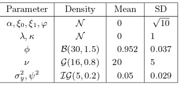
Table 2. Prior densities,means,and standard deviations.
Parameter Density Mean SD
α, ξ0, ξ1, ϕ N 0 √10
λ, κ N 0 1
φ B(30,1.5) 0.952 0.037
ν G(16,0.8) 20 5
σy2, ψ2 IG(5,0.2) 0.05 0.029
(2009) showed that in the case of the YJ transformation family, the performance of the λposterior simulations appears to be quite robust.
Next, the MCMC algorithm is run for 15,000 iterations using code written in Matlab, where the first 5,000 draws are discarded as a burn-in period. From the resultingN = 10,000 draws for each parameter, we calculate the posterior means, SDs, 95% and 92.5% highest posterior density (HPD) interval, and Geweke’s (1992) convergence diagnostic (G-CD) statistics on the initial 10% and the last 50% of the draws. To find out how fast our Markov chain converges to its stationary distribution regardless of the initial state, we estimate a quantity so called the inefficiency factor (IF). IF can be roughly interpreted as the number of MCMC iterations required to produce independent draws. When the IF is equal tom, we need to draw MCMC samplesmtimes as many as the number of uncorrelated samples. Avalue of one indicates that the draws are uncorrelated while large values indicate a slow mixing. In this study, the IF is particularly estimated as the numerical variance (square of numerical standard error) of the sample mean from the MCMC sampling scheme divided by the variance of the posterior sample mean, where the numerical standard error is computed using a Parzen window (see Kim et al. (1998) for details) with a bandwidth of 10% of the simulated draws.
Table 3. Tuning parameters for the HMC and RMHMC implementations in the R-NASV models. NFPI and AcR denote the number of fixed point iterations and acceptance rate, respectively,which has been measured every 100 iterations for 15,000 iterations.
Parameter of algorithm Parameter of model
λ φ ν z h
NL 100 6 10 6 100
∆τ 0.001 0.5 0.5 0.5 0.01
NFPI — 5 5 5 —
AcR 0.97–1.00 0.77–0.99 0.93–1.00 1.00 0.92–1.00
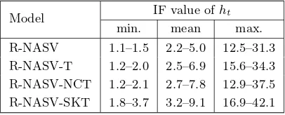
Table 4. The range of IF values for latent volatilitieshtin the HMC sampler on the R-NASV models using all data sets. The statistics have been measured for applying all transformations families,RV estimators,and data sets.
Model IF value ofht
min. mean max.
R-NASV 1.1–1.5 2.2–5.0 12.5–31.3 R-NASV-T 1.2–2.0 2.5–6.9 15.6–34.3 R-NASV-NCT 1.2–2.1 2.7–7.8 12.9–37.5 R-NASV-SKT 1.8–3.7 3.2–9.1 16.9–42.1
leapfrog iterations NL. In addition, the RMHMC implementation requires a
number of fixed point iterations. Abad choice of these parameters may result in slow mixing or incur a high computational cost in the algorithm. The selection of parameter values is particularly problematic, and there is no general guidance on how these values might best be chosen. Therefore, we tune our choices based on their acceptance rate and IF estimate from preliminary MCMC runs. Table 3 presents the parameter values used in our HMC and RMHMC implementations, in which optimal acceptance probabilities are achieved.
With the above MCMC setup, we checked the mixing performance of the samplers. In Table 4, we report the range of minimum, mean, and maximum of IF values for the estimatedhtseries in all cases. The results show that the IFs are
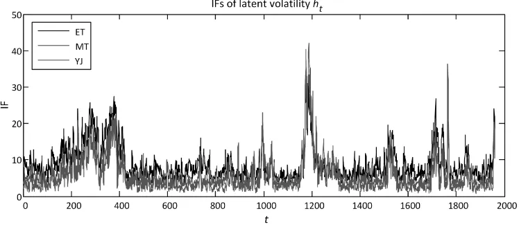
quite small, typically less than 50, suggesting that the sampler is highly efficient. For example, the IF plot for the latent volatility series of the R-MTASV-SKT model obtained using RV1HL 2004–2011 is displayed in Fig. 4. Thus, the HMC sampler can reliably estimate all latent variables in the R-NASV models.
Figure 4. IF plots for latent volatilityhtof the R-NASV-LSKT models obtained using RV1HL
2004–2011.
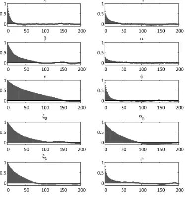
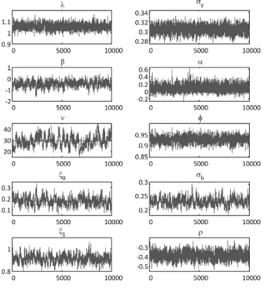
The autocorrelation and trace plots of the posterior samples for the R-MTASV-SKT model adopting RV1HL over the time period 2004–2011 are dis-played in Figs. 5 and 6, respectively. The autocorrelation plots show quick decay of the autocorrelation as time lag between samples increases, indicating that the process is stationary. Trace plots of samples indicate that the chains fluctuate to be around their means, indicating that chains could have reached the right distri-bution. We can conclude that the mixing of chains is quite good here. Thus, the HMC and RMHMC samplers can reliably estimate parameters in the R-NASV models.
In addition, all empirical results were obtained via implementation of code in MATLAB 2011b (running in Microsoft Windows 7), on a desktop computer incorporating an Intel Xeon 3.47GHz hexa-core CPU with 16GB RAM. The real computational time for the MCMC is approximately two, nine, and eight minutes for the models with ET, MT, and YJ specifications, respectively, when using the 2004–2007 data and approximately five, seventeen, and fifteen minutes for the models with ET, MT, and YJ specifications, respectively, when using the 2004–2011 data.
5.3. Parameter estimates
In this subsection, we concentrate on the key parameters that build the extension models. Tables 5 and 6 summarize the posterior simulation results of parameters in the R-NASV-NCT and R-NASV-SKT models for the 1-minute RV data set. These are derived from the models with a value of λcorresponding to no transformation that does not lie in 92.5% HPD interval. The posterior results for the other RV data sets are not presented because of space constraints.
Figure 5. Autocorrelation functions of samples for the R-MTASV-SKT model adopting RV 1-min over the time period 2004–2011.
mean and HPD interval ofλfor helping determine which transformation is suit-able for the data. First, the posterior mean of λ appears to suggest that the assumption of no transformation in the lagged log volatility series is firmly re-jected for all R-NASV models in each period and RV data. This result indicates that the proposed transformations are more suitable than a logarithmic trans-formation to transform the lagged log volatility series using a certain specified λ.
Figure 6. Trace plots of samples for the R-MTASV-SKT model adopting RV 1-min over the time period 2004–2011.
Table 5. Summary of the posterior sample of parameters in the R-NASV models with general-ized Student’st-distributions adopting RV1HL 2004–2007 data. LB and UB denote lower and upper bounds of HPD interval,respectively.
Statistic λ µ ν ξ0 ξ1 σy α φ σh ρ
R-ETASV-NCT model
Mean −0.037 0.069 23.89 0.088 0.853 0.277 −0.055 0.940 0.204 −0.426 SD 0.020 0.032 4.91 0.045 0.055 0.009 0.147 0.011 0.016 0.056 95% LB −0.077 0.043 15.55 −0.000 0.749 0.259 −0.345 0.918 0.169 −0.538 92.5% LB −0.074 0.146 15.78 0.008 0.752 0.260 −0.320 0.920 0.174 −0.528 92.5% LB −0.002 0.129 32.65 0.170 0.950 0.294 0.196 0.959 0.234 −0.327 95% UB 0.002 0.130 34.28 0.179 0.964 0.297 0.233 0.961 0.236 −0.318 IF 3.9 1.5 85.4 84.8 58.2 11.5 6.2 6.2 65.9 19.3 R-YJASV-NCT model
Mean 0.942 0.069 23.90 0.088 0.854 0.276 −0.035 0.939 0.205 −0.424 SD 0.029 0.032 4.67 0.043 0.059 0.009 0.147 0.011 0.019 0.057 95% LB 0.883 0.006 15.46 0.006 0.742 0.257 −0.325 0.917 0.168 −0.534 95% UB 0.998 0.133 33.71 0.175 0.973 0.295 0.263 0.962 0.244 −0.308 IF 3.5 1.5 62.8 37.9 64.8 12.8 4.8 8.1 79.7 19.2
Statistic λ β ν ξ0 ξ1 σy α φ σh ρ
R-ETASV-SKT model
Mean −0.037 −0.436 24.12 0.099 0.858 0.278 0.027 0.940 0.203 −0.446 SD 0.020 0.319 4.51 0.048 0.058 0.009 0.140 0.011 0.017 0.057 95% LB −0.080 −1.099 16.01 0.008 0.740 0.260 −0.256 0.917 0.169 −0.560 92.5% LB −0.075 −1.005 16.72 0.016 0.753 0.262 −0.215 0.919 0.171 −0.545 92.5% UB −0.001 0.140 32.28 0.190 0.962 0.295 0.278 0.961 0.235 −0.341 95% UB 0.002 0.178 33.29 0.201 0.968 0.296 0.292 0.963 0.239 −0.336 IF 4.9 47.2 70.5 73.1 72.0 10.1 10.6 7.6 64.3 15.3 R-YJASV-SKT model
Mean 0.942 −0.444 23.35 0.103 0.862 0.278 0.039 0.939 0.202 −0.446 SD 0.029 0.306 4.82 0.045 0.054 0.009 0.139 0.011 0.016 0.058 95% LB 0.883 −1.028 13.88 0.017 0.759 0.259 −0.228 0.916 0.170 −0.555 92.5% LB 0.890 −0.981 14.56 0.023 0.768 0.261 −0.203 0.918 0.173 −0.547 92.5% UB 0.996 0.109 31.45 0.186 0.960 0.295 0.295 0.959 0.231 −0.343 95% UB 1.000 0.183 32.7 0.194 0.970 0.296 0.326 0.961 0.234 −0.330 IF 4.0 46.4 89.8 44.9 50.7 12.1 9.4 10.2 46.0 18.6
non-linear specifications seem to underestimate the HPD intervals. In the model adopting RV5HL and TSRV5HL, the result is statistically significant for the MT specification only. Furthermore, we found that the 95% HPD intervals computed from the MT specification are slightly overestimated. Thus, the TOPIX data provide significant evidence in support of some power transformations when the 92.5% and 95% HPD intervals are considered.
Table 6. Summary of the posterior sample of parameters in the R-NASV models with gener-alized Student’st-distributions adopting RV1HL2004–2011 data.
Statistic λ µ ν ξ0 ξ1 σy α φ σh ρ
R-ETASV-NCT model
Mean 0.016 0.026 28.97 0.161 0.898 0.302 0.046 0.947 0.233 −0.365 SD 0.008 0.023 4.71 0.034 0.037 0.008 0.121 0.008 0.014 0.040 95% LB −0.001 −0.016 19.81 0.098 0.827 0.287 −0.189 0.931 0.206 −0.446 92.5% LB 0.001 −0.014 20.70 0.102 0.835 0.288 −0.173 0.932 0.208 −0.440 92.5% UB 0.032 0.066 37.29 0.223 0.965 0.317 0.257 0.961 0.259 −0.259 95% UB 0.033 0.073 38.10 0.231 0.969 0.319 0.285 0.963 0.261 −0.287 IF 3.3 1.4 94.8 66.8 65.4 13.0 3.9 6.6 59.3 13.5 R-MTASV-NCT model
Mean 1.054 0.027 28.60 0.169 0.893 0.302 0.083 0.927 0.235 −0.365 SD 0.028 0.022 5.18 0.030 0.034 0.007 0.086 0.016 0.014 0.040 95% LB 0.998 −0.017 20.20 0.103 0.831 0.288 −0.081 0.897 0.208 −0.443 92.5% LB 1.005 −0.015 20.65 0.106 0.834 0.289 −0.064 0.901 0.209 −0.436 92.5% UB 1.102 0.065 38.07 0.218 0.953 0.317 0.249 0.958 0.258 −0.297 95% UB 1.104 0.072 39.58 0.225 0.964 0.319 0.267 0.960 0.262 −0.290 IF 10.7 1.0 83.4 42.8 39.5 10.0 4.2 11.6 38.2 10.9
Statistic λ β ν ξ0 ξ1 σy α φ σh ρ
R-ETASV-SKT model
Mean 0.016 −0.513 29.34 0.185 0.907 0.304 0.059 0.948 0.230 −0.383 SD 0.008 0.321 4.78 0.036 0.037 0.008 0.117 0.007 0.013 0.041 95% LB −0.001 −1.149 20.00 0.117 0.833 0.288 −0.159 0.934 0.202 −0.464 92.5% LB 0.000 −1.052 20.82 0.119 0.843 0.290 −0.150 0.935 0.205 −0.458 92.5% UB 0.030 0.066 39.71 0.242 0.974 0.318 0.263 0.962 0.254 −0.312 95% UB 0.032 0.083 40.38 0.253 0.979 0.319 0.300 0.964 0.256 −0.305 IF 2.9 61.0 89.3 78.5 54.6 12.3 4.1 6.8 58.2 21.2 R-MTASV-SKT model
Mean 1.056 −0.474 29.00 0.177 0.910 0.304 0.102 0.927 0.228 −0.389 SD 0.027 0.283 4.70 0.038 0.035 0.007 0.082 0.016 0.014 0.041 95% LB 1.005 −1.000 20.50 0.106 0.845 0.289 −0.057 0.897 0.201 −0.469 95% UB 1.111 0.113 38.36 0.256 0.987 0.320 0.267 0.959 0.255 −0.309 IF 13.0 37.6 102.9 54.9 49.6 9.3 10.9 12.6 48.4 15.3 R-YJASV-LSKT model
data is smaller than the corresponding value in the 2004–2007 data.
Regarding the non-linear bias correction parameter of the RV equation, ξ1 deviated from the assumption of Takahashiet al.(2009) thatξ1 = 1 when apply-ing the RV1HL and BV1HL estimators. Even the upper limit of the 98% HPD interval of ξ1 was less than one (result not shown). We note that the deviation from 1 tends to be larger as the variance decreases from approximately 0.12. So the proposed models provide a log RV persistence of less than one using the RV estimators based on a sampling at very high frequency. This finding is consistent with the empirical evidence found by Hansenet al. (2011) and Takahashi et al. (2014) when applying a realized kernel estimator.
We next consider the posterior evidence regarding parameters of generalized Student’st-error distributions. Deviation of returns from the normality assump-tion is expressed by the ν, µ, and β parameters. The posterior means of the degrees of freedom ν are considerably higher than 8 (between 23 and 26 for the 2004–2007 data and between 27 and 31 for the 2004–2011 data), indicating skewness and kurtosis (see Aas and Haff (2006) for explanation). In the NCT specification, the results show that the 2004–2007 data favor the NCT distribu-tion since the 95% HPD interval ofµexcludes 0. We even found that the posterior probability thatµis positive is greater than 0.98 (result not shown). Meanwhile, although the 90% HPD intervals ofµ in the model with NCT specification over the time period 2004–2011 include 0 (result not shown), their posterior distribu-tions are largely positive as shown in Fig. 7 (first row) for the model with the MT specification. Considering the SKT specification, the measure of skewness expressed byβ shows that all data do not favor the SKT specification since the HPD interval includes 0 when the 90% HPD interval of β is considered (result not shown). The only exception is the model adopting RV1HL over the time
riod 2004–2011. In contrast to the empirical results from Takahashiet al.(2014), our returns data provide strong evidence in support of skewness over both time periods, where the deviation of β from zero is relatively large. In fact, posterior distributions ofβ in the SKT specification are largely negative as shown in Fig. 7 (second row) for the model with the MT specification. Those results present ev-idence of generalized Student’s t-error distributions in both data sets using all four RVs.
Finally, we observe the performance of persistence φ. Since the assumption of stationary has been made in the prior selection ofφ, its posterior mean as well as its confidence interval deviate from the non-stationary assumption. Further-more, we found that the highest persistence in the non-linear volatility process is provided by the MT specification in the 2004–2007 data and by the YJ spec-ification in the 2004–2011 data. Compared with the linear version, our results show that the non-linear volatility process with ET and YJ specifications in each period and with the MT specification in the 2004–2011 data is less persistent. 5.4. Model selection
This section investigates whether the data better support the linear or non-linear volatility processes to improve the model fit. To determine the best trans-formation, we compute marginal likelihoods using the Gelfand and Dey (1994) and Geweke (1999) numerical procedures, as explained in Section 4. Tables 7 and 8 present the values of the Bayes factor for the R-NASV models against the R-ASV models and the models with SKT distribution against competing models. From Table 7, we found that the log Bayes factors for the R-NASV models against the ASV models are greater than 3 in all cases, indicating that the R-NASV models provide the best fit. In fact, the log Bayes factors provide strong
Table 7. Logarithmic Bayes factors of the R-NASV models against the R-ASV models on the same returns distribution evaluated in the TOPIX data set.
R-ANSV vs R-ASV
RV Transformation SKT NCT T normal SKT NCT T normal
TOPIX 2004–2007 TOPIX 2004–2011
RV1
ET 7.78 10.94 6.88 5.50 3.89 5.43 4.66 4.70
MT 3.68 4.20 5.44 4.91 8.38 9.92 10.70 7.99
YJ 10.12 11.78 7.68 8.09 4.50 7.75 9.40 6.88
RV5
ET 13.65 10.97 12.30 12.55 9.71 6.95 11.02 3.94
MT 10.13 3.39 3.55 5.15 21.38 12.45 16.93 12.26
YJ 11.64 8.03 9.23 9.82 11.36 9.06 12.35 5.30
BV1
ET 22.88 9.53 12.21 22.13 5.66 23.25 13.79 13.15
MT 19.96 4.20 8.19 13.64 8.78 24.57 15.84 21.56
YJ 38.47 10.89 8.93 15.70 5.32 22.94 6.11 11.11
TSRV5
ET 11.76 5.30 15.59 19.09 11.47 7.83 6.06 3.19
MT 3.92 4.95 6.46 14.07 18.78 11.01 9.05 10.44
and very strong evidence in support of power transformations of the lagged log volatility rather than no transformation in the R-ASV models.
When the three competing R-NASV models are compared over the time period 2004–2007, there is no clear pattern to determine which transformation is the best in all returns distribution specifications (indicated by the largest value of log Bayes factor for any RV data sets) or in all RV data sets (indicated by the largest value of log Bayes factor for any returns distributions). We note that the R-ETASV and R-YJASV models are very competitive and outperform the R-MTASV model. The YJ and ET specifications are suggested in the models adopting RV1HLand RV5HL, respectively. In both models adopting BV1HLand TSRV5HL, the YJ and ET specifications rank first for the model accommodating generalized Student’s t-distributions and other distributions, respectively. Over the 2004–2011 data having a very high kurtosis, the R-MTASV models provide the best fit for any returns distributions and RV data sets. Those results are consistent with previously reported results in terms of a credible interval.
Comparing the results of the model using the four different returns distribu-tions in any transformation specification, see Table 8, indicates that the R-NSV model with the SKT distribution specification for returns error is the most fa-vored in each period. The log Bayes factors in favor of this specification compared with the second best fitting specification are greater than 11, which is very strong margin. Therefore, the following discussion is focused on the models with the SKT distribution.
Table 8. Logarithmic Bayes factors of the models with SKT distribution against competing models on the same transformation for lag volatility evaluated in the TOPIX data set.
Returns distribution
RV Transformation NCT T normal NCT T normal
TOPIX 2004–2007 TOPIX 2004–2011
RV1
no 26.56 32.09 39.86 13.49 18.64 30.61
ET 23.40 32.99 42.14 11.95 17.87 29.80
MT 26.04 30.33 38.63 11.95 16.32 31.00
YJ 24.86 34.49 41.85 10.24 13.74 28.23
RV5
no 14.66 20.37 30.22 27.00 33.18 37.58
ET 17.34 21.72 31.32 29.76 31.87 43.35
MT 21.40 26.95 35.20 35.93 37.63 46.70
YJ 18.27 22.78 32.04 29.30 32.19 43.64
BV1
no 13.48 23.33 41.25 33.49 39.83 51.93
ET 15.21 22.38 30.38 15.90 31.70 44.44
MT 17.62 23.48 35.95 17.70 32.77 39.15
YJ 29.49 41.30 52.45 15.87 39.04 46.14
TSRV5
no 19.11 33.37 44.47 17.01 29.85 40.22
ET 25.57 29.54 37.14 20.65 35.26 48.50
MT 18.08 30.83 34.32 24.78 39.58 48.56
For the 2004–2007 data, the R-YJASV-SKT and R-ETASV-SKT models, respectively, provide the first and second best fit to the RV1HL, BV1HL, and TSRV5HL data. Using the RV5HL data, the ranking between the first and sec-ond best is reversed with the R-ETASV-SKT model becoming first. Clearly, with regard to its log Bayes factors, the R-YJASV-SKT model is very strongly favored for the BV1HL data, positively favored for the RV1HL data, and fairly insignificant for the TSRV5HL data. With the RV5HL data, the R-ETASV-SKT model against the R-YJASV-SKT model is positively favored. Furthermore, the evidence in favor of the poorest fitting model of the R-NASV-SKT models, the one having the MT specification, compares strongly with the R-ASV-SKT model in the RV1HL and TSRV5HL cases and is also very strong in the RV5HL and BV1HL cases.
For the 2004–2011 data, compared with the second best models, the R-MTASV-SKT model is strongly for the RV1HL and BV1HL data and very strongly favored for the RV5HL and TSRV5HL data. The ETASV and R-YJASV models are very competitive. Furthermore, the poorest fitting model of the R-NASV-SKT models compared with the R-ASV-SKT model is strongly favored in the RV1HL case and very strongly favored in the others.
5.5. Sensitivity ofpriors
Concerning the sensitivity of MCMC output to prior choices, let us recall from the previous analysis that the R-MTASV-SKT model is the best perform-ing model for the 2004–2011 data. This section applies a sensitivity test for this model on the power parameter λ. Our intention is to show that posterior
sim-Table 9. Parameter estimates ofλfor the R-MTASV-SKT using the 2004–2011 data.
Statistic Prior
N(0,1) N(0,10) U(−10,10) U(−100,100) model adopting RV1HL
Mean (SD) 1.056 (0.027) 1.058 (0.028) 1.056 (0.028) 1.056 (0.027) 90% HPD [1.012,1.102] [1.012,1.105] [1.009,1.102] [1.009,1.100]
IF 12.8 13.9 13.5 12.3
model adopting RV5HL
Mean (SD) 1.055 (0.030) 1.054 (0.030) 1.057 (0.030) 1.055 (0.030) 90% HPD [1.006,1.107] [1.003,1.103] [1.007,1.106] [1.004,1.102]
IF (NSE) 18.2 14.1 15.4 15.6
model adopting BV1HL
Mean (SD) 1.044 (0.028) 1.045 (0.029) 1.044 (0.029) 1.046 (0.028) 90% HPD [0.999,1.095] [0.995,1.090] [0.997,1.092] [0.998,1.091]
IF (NSE) 14.1 15.6 13.0 13.3
model adopting TSRV5HL
Mean (SD) 1.061 (0.030) 1.058 (0.030) 1.059 (0.029) 1.059 (0.030) 90% HPD [1.011,1.109] [1.007,1.107] [1.008,1.107] [1.010,1.109]
Figure 8. The posterior distributions for the λ parameter using various prior assumptions. These are obtained from the last 10,000 iterations of the R-MTASV-SKT model adopting RV1HLdata (2004–2011).
ulations give similar characteristics in terms of the mean, standard deviation, credible interval, and sampling efficiency estimates under alternative priors ofλ. In the previous estimation, we used a normal prior for λ with variance 1. To study the sensitivity of the estimation results to the diffuse prior on λ, we first choose the same normal prior but we increase the variance to a value of 10. We then choose the uniform priors on [−10,10] and [−100,100]. Notice that the standard deviation for the last two consecutive priors are 33.33 and 833.33. The estimates for all parameters are found to be almost the same under all priors. In particular, the parameter estimates and sampling efficiency forλare reported in Table 9. It shows that the estimates for all parameters in the model are not affected by changing the prior forλ. To graphically illustrate our results, Fig. 8 displays the sample paths and posterior distributions for theλusing all four prior assumptions.
6. Conclusions and extensions
inter-val although Takahashi et al.(2014) showed that this additional bias correction does not improve the model fit. The performance of competing models was quan-tified by the logarithm of estimated marginal likelihood. The estimation results demonstrated that the model with the SKT distribution best fitted the TOPIX data, although the skewness parameter in some of the models is not fully guaran-teed by the 90% HPD interval. Furthermore, the marginal likelihood and Bayes factor criterion indicate that the proposed R-NASV model outperforms the RSV model, where the three competing R-NASV models are very competitive.
The proposed R-NASV models could also be extended by considering a class of non-linear transformations for RV. Gon¸calves and Meddahi (2011) particularly showed that the log transformation of RV can be improved upon by choosing values for the BC parameter other than zero.
Acknowledgements
The authors wish to thank Dr. Shuichi Nagata for some Matlab codes and helpful discussions.
References
Aas, K. and Haff, I. H. (2006). The generalized hyperbolic skew Student’st-distribution,Journal of Financial Econometrics,4, 275–309.
Andersen, T. G., Bollerslev, T., Diebold, F. X. and Labys, P. (2001). The distribution of realized exchange rate volatility,J. Am. Stat. Assoc.,96(453), 42–55.
Andersen, T. G., Bollerslev, T. and Diebold, F. X. (2005). Roughing It Up: Including Jump Components in the Measurement, Modeling and Forecasting of Return Volatility, Working Paper Series 11775, National Bureau of Economic Research.
Barndorff-Nielsen, O. E. (1977). Exponentially decreasing distributions for the logarithm of particle size,Proc. R. Soc. Lond.,Ser. A,353(1674), 401–419.
Barndorff-Nielsen, O. E. and Shephard, N. (2004). Power and bipower variation with stochastic volatility and jumps,Journal of Financial Econometrics,2(1), 1–37.
Barndorff-Nielsen, O. E., Hansen, P., Lunde, A. and Shephard, N. (2008). Designing realised kernels to measure the ex-post variation of equity prices in the presence of noise, Econo-metrica,76, 1481–1536.
Bollerslev, T. (1986). Generalized autoregressive conditional heteroskedasticity, J. Econom.,
31, 307–327.
Box, G. E. P. and Cox, D. R. (1964). An analysis of transformations,J. R. Stat. Soc. Ser. B,
26, 211–252.
Carnero, M. A., Pea, D. and Ruiz, E. (2001). Is Stochastic Volatility More Flexible than GARCH?, Working Paper 01–08, Universidad Carlos III de Madrid. Retrieved from http://e-archivo.uc3m.es/bitstream/10016/152/1/w
Chen, M. H. and Shao, Q. M. (1999). Monte Carlo estimation of Bayesian credible and HPD intervals,J. Comput. Graph. Stat.,8, 69–92.
Dobrev, D. and Szerszen, P. (2010). The Information Content of High-Frequency Data for Esti-mating Equity return Models and Forecasting Risk, Working Paper, Finance and Economics Discussion Series.
Engle, R. F. (1982). Autoregressive conditional heteroskedasticity with estimates of the variance of the united kingdom inflation,Econometrica,50, 987–1007.
Geweke, J. (1992). Evaluating the accuracy of sampling-based approaches to the calculation of posterior moments,Bayesian Statistics 4 (eds. J. M. Bernardo, J. O. Berger, A. P. Dawid and A. F. M. Smith), pp. 169–194 (with discussion), Clarendon Press, Oxford, UK. Geweke, J. (1993). Bayesian treatment of the independent student-t linear model, J. Appl.
Econ.,8, S19–S40.
Geweke, J. (1999). Using simulation methods for Bayesian econometric models: Inference, development, and communication,Econom. Rev.,18(1), 1–73.
Geweke, J. and Whiteman, C. (2006). Bayesian forecasting,Handbook of Economic Forecasting
(eds. G. Elliott, C. W. J. Granger and A. Timmermann), pp. 3–80, Elsevier B. V.
Ghysels, E., Harvey, A. C. and Renault, E. (1996). Stochastic volatility, Handbook of Statis-tics: Statistical Methods in Finance (eds. G. S. Maddala and C. R. Rao), pp. 119–191, Amsterdam: Elsevier Science.
Girolami, M. and Calderhead, B. (2011). Riemann manifold Langevin and Hamiltonian Monte Carlo methods,J. R. Stat. Soc. Ser. B,73(2), 1–37.
Gon¸calves, S. and Meddahi, N. (2011). Box-Cox transforms for realized volatility,J. Econom.,
160, 129–144.
Hansen, P. R. and Lunde, A. (2005). A forecast comparison of volatility models: Does anything beat a GARCH(1,1),J. Appl. Econ.,20(7), 873–889.
Hansen, P. R., Huang, Z. and Shek, H. H. (2011). Realized GARCH: A joint model for returns and realized measures of volatility,J. Appl. Econ.,27(6), 877–906.
Harvey, A. C. and Shephard, N. (1996). The estimation of an asymmetric stochastic volatility model for asset returns,J. Bus. Econ. Stat.,14, 429–434.
Jacquier, E. and Miller, S. (2010). The Information Content of Realized Volatility, Working Paper HEC Montreal.
Jacquier, E., Polson, N. G. and Rossi, P. E. (2004). Bayesian analysis of stochastic volatility models with fat-tails and correlated errors,J. Econom.,122(1), 185–212.
John, J. A. and Draper, N. R. (1980). An alternative family of transformations,Applied Statis-tics,29, 190–197.
Johnson, N. L., Kotz, S. and Balakrishnan, N. (1995). Continuous Univariate Distributions
(2nd ed.), John Wiley & Sons.
Kass, R. E. and Raftery, A. E. (1995). Bayes factors,J. Am. Stat. Assoc.,90(430), 773–795.
Kim, S., Shephard, N. and Chib, S. (1998). Stochastic volatility: Likelihood inference and comparison with ARCH models,Stochastic Volatility:Selected Readings (ed. N. Shephard), Oxford University Press.
Koop, G. M., Poirier, D. J. and Tobias, J. L. (2007). Bayesian Econometric Methods, Cambridge University Press.
Koopman, S. J. and Scharth, M. (2013). The analysis of stochastic volatility in the presence of daily realized measures,Journal of Financial Econometrics,11(1), 76–115.
Manly, B. F. (1976). Exponential data transformation,The Statistician,25, 37–42.
Marwala, T. (2012). Condition Monitoring Using Computational Intelligence Methods, Springer-Verlag.
Nakajima, J. and Omori, Y. (2012). Stochastic volatility model with leverage and asymmetri-cally heavy-tailed error using GH skew Student’st-distribution,Comput. Stat. Data Anal.,
56, 3690–3704.
Neal, R. M. (2011). MCMC using Hamiltonian dynamics, Handbook of Markov Chain Monte Carlo (eds. S. Brooks, G. A., G. Jones and X.-L. Meng), pp. 113–162, Chapman & Hall / CRC Press.
Takahashi, M., Omori, Y. and Watanabe, T. (2009). Estimating stochastic volatility models using daily returns and realized volatility simultaneously, Comput. Stat. Data Anal., 53,
2404–2426.
Takahashi, M., Omori, Y. and Watanabe, T. (2014). Volatility and Quantile Forecasts by Real-ized Stochastic Volatility Models with GeneralReal-ized Hyperbolic Distribution, Working Paper Series CIRJE-F-921, CIRJE, Faculty of Economics, University of Tokyo.
Takaishi, T. (2009). Bayesian inference of stochastic volatility model by Hybrid Monte Carlo,
Taylor, S. J. (1982). Financial returns modelled by the product of two stochastic processes—a study of the daily sugar prices 1961–75, Stochastic Volatility: Selected Readings (ed. N. Shephard), pp. 60–82, Oxford University Press, New York.
Tsiotas, G. (2009). On the use of non-linear transformations in Stochastic Volatility models,
Statistical Methods and Applications,18, 555–583.
Tsiotas, G. (2012). On generalised asymmetric stochastic volatility models,Comput. Stat. Data Anal.,56, 151–172.
Watanabe, T. and Asai, M. (2001).Stochastic Volatility Models with Heavy-Tailed Distributions:
A Bayesian Analysis, Bank of Japan, IMES Discussion Paper Series No. 2001-E-17. Weisberg, S. (2014). Yeo-Johnson Power Transformations, Working Paper Series CIRJE-
F-921, CIRJE, Faculty of Economics, University of Tokyo.
Yeo, I.-K. and Johnson, R. (2000). A new family of power transformations to improve normality or symmetry,Biometrika,87(4), 954–959.
Yu, J. (2002). Forecasting volatility in the New Zealand stock market, Appl. Financ. Econ.,
12, 193–202.
Yu, J. (2005). On leverage in a stochastic volatility model,J. Econom.,127(2), 165–178.
Zhang, L., Mykland, P. A. and A¨ıt-Sahalia, Y. (2005). A tale of two time scales: Determining integrated volatility with noisy high-frequency data,J. Am. Stat. Assoc.,100(472), 1394–