El e c t ro n ic
Jo ur n
a l o
f P
r
o ba b i l i t y
Vol. 5 (2000) Paper no. 14, pages 1–40.
Journal URL
http://www.math.washington.edu/~ejpecp/ Paper URL
http://www.math.washington.edu/~ejpecp/EjpVol5/paper14.abs.html
TRAVELLING WAVES FOR A CERTAIN FIRST-ORDER COUPLED PDE SYSTEM Owen D. Lyne
School of Mathematical Sciences, University of Nottingham University Park, Nottingham, NG7 2RD, United Kingdom
Abstract. This paper concentrates on a particular first-order coupled PDE system. It provides both a detailed treatment of theexistenceanduniquenessof monotone travelling waves to various equilibria, by differential-equation theory and by probability theory and a treatment of the corresponding hyperbolic initial-value problem, by analytic methods.
The initial-value problem is studied using characteristics to show existence and uniqueness of a bounded solution for bounded initial data (subject to certain smoothness conditions). The concept ofweak so-lutions to partial differential equations is used to rigorously examine bounded initial data with jump discontinuities.
For the travelling wave problem the differential-equation treatment makes use of a shooting argument and explicit calculations of the eigenvectors of stability matrices.
The probabilistic treatment is careful in its proofs ofmartingale(as opposed to merely local-martingale) properties. A modernchange-of-measuretechnique is used to obtain the best lower bound on the speed of the monotone travelling wave — with Heaviside initial conditions the solution converges to an approximate travelling wave of that speed (the solution tends to one ahead of the wave-front and to zero behind it). Waves to different equilibria are shown to be related by Doob h-transforms. Large-deviation theory
provides heuristic links between alternative descriptions of minimum wave speeds, rigorous algebraic proofs of which are provided.
Key words. Travelling waves. Martingales. Branching processses AMS Classification. 35L35; 60J27; 60G44
1
Introduction
Connections between parabolic and elliptic equations and diffusion processes are well-known. In this paper we explore the connections between hyperbolic partial differential equations and stochastic processes by treating the following system.
Let r1, r2, q1, q2 be positive (since they correspond to rates of probabilistic processes) constants and b1, b2 unrestricted real constants, fixed throughout. Let θ be a positive rate parameter. We consider an equation system related to the generalized FKPP system discussed in Champneys, Harris, Toland, Warren and Williams [2]. Here the system of interest is
∂u ∂t =B
∂u ∂x+R(u
2
−u) +θQu, (1)
where u is a vector-valued function from [0,∞)×R to R
2, u= (u
1, u2) ∈ R
2 and u2 = (u2
1, u22), and where
B :=
b1 0 0 b2
, R:=
r1 0
0 r2
, Q:=
−q1 q1 q2 −q2
.
(We use ‘:=’ to mean ‘is defined to equal’.)
Dunbar [8] considered a similar system but with q1 = q2, r1 = r2 and the nonlinearity was 14(u1 +
u2)2
1 1
rather thanu2. Holmes [10] compared reaction-diffusion systems to reaction-telegraph models (again with symmetry in the nonlinearity in both terms) for animal movement; if equation (1) is rewritten as a single second-order PDE it can be seen that our system is a reaction-telegraph model, though we find it more convenient to work with the pair of first-order equations. Hadeler [9] discussed more general non-linearities but still retained the conditionq1 = q2. We contrast the probabilistic interpretation of these models and ours in section 1.4.
A travelling-wave solution of equation (1) is a solution of the formu(t, x) :=w(x−ct) (where w:R→ R
2). wdescribes a travelling wave if and only if
(B+cI)w′+R(w2−w) +θQw= 0. (2)
The ‘source point’ S = (0,0) and the ‘target point’ T = (1,1) are clearly equilibria of equation (2). If r1r2≥4θ2q1q2, there will also be equilibria at the two points
E±=
1
2 +θρ1±
√
∆,1
2 +θρ2∓
√
∆
,
whereρi:=qi/ri and ∆ := 14−θ2ρ1ρ2.
Forθ∈(0,∞) we study the existence of monotone travelling waves fromS toT. Waves fromS to the other equilibria can be obtained through a transformation detailed in section 1.3. Monotone travelling waves from S to T have a direct probabilistic interpretation which we will explore in this paper, but whether such an intepretation of other travelling waves is possible is unclear.
1.1
Stability of equilibria
Suppose that (B+cI) is invertible and write equation (2) in the form dw
dx =F(w). (3)
Then F is a quadratic polynomial. Let E be an equilibrium point of (2), thus F(E) = 0. Then write w(x)−E=v(x) and expand equation (3) to first order inv. This yields
dv
dx =K(E)v, Kij(E) := ∂Fi
∂wj
ThusKc,θ(T) (we writeKc,θ to emphasize the dependence onc andθ) satisfies
(B+cI)Kc,θ(T) +R+θQ= 0 (4)
andKc,θ(S) satisfies
(B+cI)Kc,θ(S)−R+θQ= 0.
The stability properties of these matrices are investigated in section 3.
1.2
The main ODE theorem
DEFINITION. An eigenvalue λ of a real 2×2 matrix M will be called stable [respectively, unstable]
monotoneif
(i)λis real and negative [positive], and
(ii)M has an eigenvector (v1, v2) corresponding toλwithv1v2≥0.
This definition links nicely with the Perron-Frobenius Theorem (see Seneta [15]). The theorem implies that a square matrix M with all off-diagonal entries strictly positive has a special eigenvalue ΛP F(M)
with an associated eigenvector with all entries positive and such that every other eigenvalue of M has real part less than ΛP F(M). Moreover, any eigenvector with all entries positive must be a multiple of the
Perron-Frobenius eigenvector.
As will be proven in section 3 (Lemma 3.1), for any fixedθ >0, there exists a critical valuec(θ) in the interval min(−b1,−b2)≤c(θ)≤max(−b1,−b2) — with the property that ifc > c(θ),c6= max(−b1,−b2), thenKc,θ(T) has at least one stable monotone eigenvalue, and if c < c(θ), c6= min(−b1,−b2), it has no such eigenvalues. Since a necessary condition for the existence of a monotone travelling wave of (2) which converges toT asx→ ∞is the existence of a stable monotone eigenvalue ofKc,θ(T) this provides a lower
bound on possible values ofcfor which a monotone travelling wave can exist. It is shown later that this condition oncis also sufficient for the existence of a monotone connection from S toT, see section 4.5. Large-deviation theory gives probabilistic heuristics for this critical value, see section 5.2. Thus we can state our main result as follows.
Theorem 1.1 Suppose that c > c(θ), then there exists one and, modulo translation, only one monotone solution of equation (2) with w(x)→S asx→ −∞ andw(x)→T asx→+∞. For c < c(θ) there is no such solution.
This theorem is proven in section 4 using a shooting argument. Behaviour atc(θ) itself depends on the relative values of parameters as follows (these special cases are detailed in section 4.6):
• If c(θ) is in the interval min(−b1,−b2)< c(θ)<max(−b1,−b2) then there is a unique, monotone solution forc=c(θ);
• For i = 1,2, if c(θ) = −bi, then there is a unique monotone solution forc = c(θ) if and only if
θqi=ri.
1.3
A Doob
h
-transform
Lemma 1.2 Suppose that θ is fixed at a value where ∆≥0, so thatE+ andE− exist. If E= (α1, α2)
denotes eitherE+ orE−, then the substitution
˜
qi :=qiαj/αi (j6=i), r˜i:=riαi, u˜i:=ui/αi, w˜i:=wi/αi (5)
transforms (1) and (2) into their ∼ versions, monotone waves from S to E for the original problem corresponding exactly to monotone waves from S toT for the ∼problem. The possibility that E+=E− and∆ = 0is not excluded.
Much of our work therefore automatically transfers to the case whenT is replaced byE+orE−, though
the critical valuesc±(θ) ofθcorresponding to waves fromS toE± will be different.
1.4
Key probability theorems
Our aim in section 5 will be to prove the following theorems which connect a probability model, defined below, with the system (1). Note that we often switch between two equivalent notations in the probability part of this paper to reduce the use of subscripts. Thus we will sometimes write, for example, b(y) for by,w(x, y) forwy(x) andu(t, x, y) foruy(t, x) (fory= 1,2).
LetI :={1,2}and consider the following two-type branching system of particles. At time t≥0, there areN(t) particles, thek-th particle — in order of birth— having positionXk(t) inR andtypeYk(t) in I. Thestateof the system at timet is therefore
N(t);X1(t), . . . , XN(t)(t);Y1(t), . . . , YN(t)(t)
. (6)
Particles, once born, behave independently of one another. Each particle lives forever. The type of a particle (once born) is an autonomous Markov chain onI withQ-matrixθQ. While a particle is of type y∈I, it moves with constant velocityb(y), and it gives birth —to one child each time, at its own current position and of its own current type— in a Poisson process of rater(y). So,r(y) is the breeding rate of typey.
The branching system in Dunbar [8] hadq1 =q2, r(1) =r(2) and particles, rather than giving birth to one particle of the same type and living on themselves, die and give birth to two particles of independent
random types, with each having equal probability of being of either type. The equations studied by Hadeler [9] correspond to the new pair of particles having type correlated to that of their parents, for any correlation except±1. Our model permitsq16=q2, so that the particle-type Markov Chain can have any equilbrium distribution onI
For our model it makes no difference whether you consider that one new particle has been born and the old one lives on too, or that two new particles of the same type are born. However, when the type of the new particles is random, this distinction is crucial. Our model is thus distinct from those previously considered.
WritePx,y(with associated expectationEx,y) for the law of this process when it starts from one particle of typeY1(0) =y at positionX1(0) =x. By martingale [respectively, local martingale, supermartingale, ...] we mean a process which is for everyPx,y a martingale [respectively, ...] relative to the natural filtration
Ft(Px,y-augmented, to be precise) of the process at (6). The state-space for this process is
S:= [
n≥1
{n} ×R
n
×In
. (7)
Define L(t) := infk≤N(t)Xk(t). This is the position of the left-most particle. The asymptotic speed of
Theorem 1.3 As t→ ∞, the following holds almost surely(a.s.)
t−1L(t)→ −c(θ). (8)
Ifu satisfies the coupled system(1), fort≥0 andx∈R and if
u(0, x, y) =
1 ifx >0,
0 ifx≤0,
then fort >0,0≤u(t, x, y)≤1,u(t, x, y) =Px,y[L(t)>0], and uis an approximate travelling wave of
speedc(θ)in the sense that
u(t, x+γt, y)→
0 ifγ < c(θ),
1 ifγ > c(θ).
This theorem is proved, along with the following one, in sections 5.4 and 5.5. The theorem allows us to relate the speed of the spread of the particles in the probabilistic model with the wave speed of travelling waves. Specifically, we are claiming that the left-most particle travels, in the limit, at the speed−c(θ), where c(θ) is the critical speed above which a unique monotone travelling wave exists and below which no such wave exists.
An analytic proof that the weak solution of (1) is between 0 and 1 for the Heaviside initial data is included in section 2.4, as well as a proof that for continuous initial data between 0 and 1 the solution remains between 0 and 1 (see Lemma 2.2 and the subsequent remarks). The work of section 2 is not necessary for the probabilistic approach to the problem but adds insight from the viewpoint of classical analysis, and vice-versa. In section 5 we show that any (smooth) solution to the coupled system (1) that is between 0 and 1 has a McKean representation. We use this representation to motivate the (probabilistic) construction of a solution for the initial-value problem with Heaviside initial data. This constructed solution is then directly verified to satisfy the appropriate equations and does remain between 0 and 1. Consider the case when X1(0) = 0 and Y1(0) = 1, that is, work with the P0,1 law: P := P0,1. The terminology —probabilisticeigenvalue ofKc,θ(T) — is a shorthand explained fully after Theorem 5.2.
Theorem 1.4 (i)Let c > c(θ). Letλbe the probabilisticeigenvalue ofKc,θ(T). Define
Zλ(t) := N(t)
X
k=1
vλ Yk(t)exp
λ
Xk(t) +ct
,
withvλ being the eigenvector (withvλ(1) = 1) corresponding toΛP F(λ), the Perron-Frobenius eigenvalue
ofλB+θQ+R. The fact thatZλ is a martingale (see the discussion after Theorem5.2) implies that
lim inf
t→∞ t
−1L(t)
≥λ−1ΛP F(λ) (a.s.).
(ii) Since Zλ(∞) exists in L1 (by Theorem5.4) and Zλ(0) = 1, we can define a measure Qλ equivalent
toPon F∞ by
dQλ/dP=Zλ(∞)onF∞, whencedQλ/dP=Zλ(t)on Ft.
Then
Mλ(t) :=Zλ(t)−1 ∂
∂λZλ(t)
defines aQλ-martingale, and
t−1Mλ(t)→0 (a.s.).
This implies that
lim sup
t→∞
t−1L(t)≤ ∂
(iii)As c↓c(θ), we have
λ−1ΛP F(λ)→ −c(θ) and ∂
∂λΛP F(λ)→ −c(θ),
so that (8)follows.
This result gives us the weaponry to prove Theorem 1.3 using martingale techniques. Note that Theo-rem 1.3 is proved using TheoTheo-rem 1.4, and that in section 5.4 we prove TheoTheo-rem 1.4 via the TheoTheo-rems and Lemmas in the preceding sections of section 5 — hence various references to Theorems of section 5 in the statement of Theorem 1.4 are not circular.
1.5
Summary chart of results
This table is intended to help keep track of the various cases determined by the values of parameters. There is no monotone travelling wave fromS toT if No appears in both right-hand columns. The inside and outside regions mentioned here are defined in section 4 where it is shown that if a monotone travelling wave exists then it lies either in an inside, or an outside region.
Number of unstable Number of stable Monotone Connection
monotone monotone through
eigenvalues atS eigenvalues atT inside region outside region
c >max(−b1,−b2) 1 1 Yes No
max(−b1,−b2)> c > c(θ) 1 2 No Yes
c(θ)> c >min(−b1,−b2) 1 0 No No
c <min(−b1,−b2) 0 0 No No
When c ∈ {−b1,−b2} the coupled system (1) becomes an ODE and an algebraic equation. The only candidate for a travelling wave fromStoT is the corresponding segment of the solution of the algebraic equation (which is a parabola) — full details of this special case are in section 4.6.
2
Existence and uniqueness results for the PDE initial-value
problem
To study the question of global existence and uniqueness of solutions to the initial-value problem for the system (1), it is convenient to change to moving coordinates (moving at a speed of 1
2(b1+b2)) and then re-scale space so that the coefficients ofuxare 1 and−1. This is possible unlessb1=b2— we deal with this case in section 2.6. We use subscript notation to represent derivatives and relabel so that the system becomes:
ut−ux= r1(u2−u) +θq1(v−u) =: f(u, v); (9)
vt+vx= r2(v2−v) +θq2(u−v) =: g(u, v). (10)
The functionsf andg are introduced to simplify notation.
We are particularly interested in the Cauchy problem for Heaviside initial data:
u(0, x) =v(0, x) =
which we study in section 2.4, but first we study the Cauchy problem withC1-initial data. The characteristics arex+t= constant, on which∂u
∂t =f(u, v) andx−t= constant, on which ∂v
∂t =g(u, v).
Integrating along the characteristics fromt= 0 to a point (T, X) gives:
u(T, X) = u(0, X+T) + Z T
0
f (u, v)(t, X+T−t) dt;
v(T, X) = v(0, X−T) + Z T
0
g (u, v)(t, X−T+t) dt.
We work in the Banach spaceC1of 2-vector-valued functionswfor whichwandw
x are continuous and
bounded for allx, in which we choose as norm|||w|||= max(||w||,||wx||), where||w||:= supx∈R|w(x)|, the usualL∞-norm. These equations can be used with the Contraction Mapping Principle to prove existence
and uniqueness of classical solutions for a short time for C1-initial data. See Courant and Hilbert [5, pages 461–471] for details.
2.1
Proofs for smooth initial data
To go from short-time existence and uniqueness of solutions to global existence and uniqueness we prove the following lemmas which give bounds on the solutions for all time (for a certain class of initial data). These bounds then allow iteration of the Contraction Mapping argument — hence local existence and uniqueness become global. This iteration is done by using the solution obtained from local existence and uniqueness, up until a small, fixed time,τ, then taking the value of this solution at timeτ as initial data, and repeating the argument. The bounds obtained in the following two lemmas allow repeated use of the sameτ at each step, rather than having to take a sequence ofτn (whose sum may converge to a finite
blow-up time), thus we obtain existence and uniqueness for all time. To set our notation, note that we will writeu(0, x) =u0(x), v(0, x) =v0(x) for−∞< x <∞.
Lemma 2.1 If 0 < u0(x), v0(x) < K ≤1 for all x, and (u0, v0) is in C1, then C1 solutions (u, v) of
equations (9), (10)satisfy0< u, v < K for all time.
Proof. Suppose, for a contradiction, that there exists a point (T, X) where (u, v) is outside the square, (0, K)2. The value of (u, v) at this point only depends on the initial data in the interval [X−T, X+T] — this is the domain of dependence (see Courant and Hilbert [5, pages 438–440]). This data determines the solution (u, v) throughout the closed triangle, which we shall denote by Ω, of (t, x)-space whose corners are (T, X),(0, X−T) and (0, X+T).
Since Ω is compact anduandv are continuous, for each of the possible violations (that is, violations of the four inequalitiesu < K,u >0,v < K andv >0) we can find afirst timeit occurs in Ω. For example, ifu≥K at some point in Ω then there exists a point (t0, x0)∈Ω such that u(t0, x0) = K and, for all (t, x) ∈Ω with t < t0, u(t, x) < K. Similarly we can find a time (and corresponding spatial position) where the first violations of u >0, v < K and v >0 occur in Ω (if such violations do occur). We can then study thefirst violation that happens, by taking the one corresponding to the minimum of these 4 times (taking the time to beT+ 1 if it does not occur in Ω). This is well-defined because we know there is at least 1 violation and at most 4.
So, consider each possible first violation in turn. Firstly, that there exists a point (t0, x0) ∈ Ω such that u(t0, x0) = K and, for all (t, x) ∈ Ω with t < t0, u(t, x), v(t, x) ∈ (0, K)2. Then consider u restricted to the characteristicx=x0+t0−tthrough (t0, x0) (which lies entirely in Ω). From (9), with u=u(t, x0+t0−t),
∂u ∂t =r1(u
2
−u) +θq1(v−u) < r1(u2−u) +θq1(K−u)
Therefore,u≤K+ (u0−K) exp(−θq1t)< K whereu0=u(0, x0+t0), for 0≤t≤t0, which contradicts u(t0, x0) =K.
Similarly, we can show thatv(t, x)< K for all (t, x)∈Ω, and we use a similar argument to show u >0 andv >0:
∂u
∂t ≥ −(r1+θq1)u, sou≥u0exp −(r1+θq1)t>0 ifu0>0.
Hence no violation occurs in Ω which is a contradiction. This completes the proof.
Lemma 2.1 allows us to prove the following:
Lemma 2.2 If 0 ≤ u0(x), v0(x) ≤K for all x, for some constant, 0 < K ≤ 1, andu0, v0 are in C1,
then there exists a unique (global)C1solution (u, v)of equations (9), (10)satisfying 0≤u, v≤K for all
time.
Proof. Consider a sequence (un, vn)(x) of initial data satisfying the conditions of Lemma 2.1, which converges inC1 to (u
0, v0)(x). That is, each (un, vn)∈C1, 0< un, vn< K, sup
x (|u0−u n
|,|v0−vn|)→0 asn→ ∞
and
sup
x
∂u0 ∂x −
∂un
∂x ,
∂v0 ∂x −
∂vn
∂x
→0 asn→ ∞.
Up to any fixed timeτ, solutions u(n)(t, x), v(n)(t, x) satisfy 0< u(n), v(n) < K by Lemma 2.1, so that, limn→∞(u(n), v(n)) = (u, v) lies in [0, K]2. The fact that this limit exists and is a unique solution is
standard (see Courant and Hilbert [5, pages 467–468]). Sinceτis arbitrary the result is true for all time.
This lemma completes the proof of global existence and uniqueness of bounded solutions for smooth initial conditions between 0 and any constant 0< K ≤ 1. This upper limit onK is the best possible, since u2−u > 0 foru > 1, so the solution tends to grow. Indeed, it is clear that for u0(x) = v0(x) identically equal to 1 +ǫ, for anyǫ >0, the solution blows up in finite time.
However it is possible to extend the above lemmas to deal with initial data below 0, since the u2−u nonlinearity will tend to push the solution up towards 0.
Lemma 2.3 If −∞< K < u0(x), v0(x)<0 for allx, and(u0, v0)is in C1, then C1 solutions (u, v)of
equations (9), (10)satisfyK < u, v <0 for all time.
Proof. We can again look for thefirst violation, this time of the four restrictionsu > K, u <0, v > K, v < 0, and look at a characteristic going through a point at which the first violation occurs.
For the caseu=K, note that
∂u ∂t =r1(u
2
−u) +θq1(v−u) > θq1(v−u) > θq1(K−u),
so thatudoes not hitK.
Foru= 0, note that, looking at the characteristic sufficiently close to the violation point (so thatu >−1)
∂u ∂t =r1(u
2
so thatudoes not hit 0 either.
Similarly forv. Thus all the contraction mapping arguments extend to all time in the same way that the bounds on data between 0 andK (for 0< K ≤1) extended existence and uniqueness in that case.
In the same way that we passed from Lemma 2.1 to Lemma 2.2 we can relax the strict inequalities in the hypotheses of Lemma 2.3 to obtain the following result.
Lemma 2.4 If −∞< K≤u0(x), v0(x)≤0 for all x, for some constantK <0, and (u0, v0)is in C1,
thenC1 solutions (u, v) of equations(9), (10)satisfyK≤u, v≤0 for all time.
Combining Lemma 2.2 and Lemma 2.4 prepares the ground for the following result.
Lemma 2.5 If K1 < u0(x), v0(x)< K2 for all x, for some constants −∞< K1≤0 and 0≤K2≤1,
and(u0, v0)is inC1, then C1 solutions (u, v)of equations(9), (10) satisfyK1< u, v < K2 for all time.
Proof. IfK1= 0 then this result is simply a restatement of Lemma 2.2, and Lemma 2.4 deals with the caseK2= 0. So, we may assume thatK1<0< K2.
For a violation such as, say, u= K1, note that, considering a section of the characteristic sufficiently close to the violation point foru <0
∂u ∂t =r1(u
2
−u) +θq1(v−u) > θq1(v−u) > θq1(K1−u),
so thatudoes not hitK1.
For u = K2, note that, considering the characteristic sufficiently close to the violation point (so that u >0)
∂u ∂t =r1(u
2
−u) +θq1(v−u) < θq1(v−u) < θq1(K2−u),
so thatudoes not hitK2.
Similarly forv, hence we are done.
Finally, again using the inequality relaxation, and noting that if the initial data is identically zero then the solution is identically zero for all time, we have:
Lemma 2.6 If K1 ≤u0(x), v0(x)≤K2 for all x, for some constants −∞< K1≤0 and 0≤K2≤1,
and(u0, v0)is inC1, then C1 solutions (u, v)of equations(9), (10) satisfyK1≤u, v≤K2 for all time.
No such result will be true for a pair of constantsK1 and K2 both strictly on the same side of zero — the solution to the initial value problem withu0 =v0 identically equal to some constant K, such that
−∞< K <1, tends monotonically to zero (see section 2.6). This fact is put together with comparison arguments in section 2.2 to give a much stronger result than Lemma 2.6.
Given bounded initial data with an upper bound no greater than 1, we can read off the appropriate values ofK1andK2 by defining:
K1 = min
0,inf
x u0(x)
,inf
x v0(x)
,
K2 = max
0,sup
x
u0(x) ,sup
x
v0(x)
Local existence of solutions with piecewise smooth initial data (i.e. continuous but with a finite number of jump discontinuities in thex-derivative) follows by approximating (in the supremum norm) piecewise smooth data by C1 data — the limiting solutions are classical except on characteristics x±t = x
0 propagating from pointsx0of discontinuity of ∂u∂x0,
∂v0
∂x.
2.2
Comparison results
Consider two solutions (u, v) and (˜u,˜v) of the equations (9),(10), withu(0, x) =u0(x),v(0, x) =v0(x), ˜
u(0, x) = ˜u0(x), ˜v(0, x) = ˜v0(x). On the characteristics of the form x+t= constant, we know that
∂u
∂t = r1(u
2−u) +θq1(v−u),
∂u˜
∂t = r1(˜u 2
−˜u) +θq1(˜v−u˜),
and similar equations forv and ˜valong the other characteristics.
Studying the difference between the solutions along a characteristicx+t= constant, we see that it obeys the equation
∂(u−u˜)
∂t = r1 (u 2
−u˜2)−(u−˜u)
+θq1 (v−˜v)−(u−u˜),
= (u−u˜) r1(u+ ˜u−1)−θq1+θq1(v−˜v).
Provided that the initial data (u0, v0) and (˜u0,v˜0) satisfies the conditions of Lemma 2.6, then (u+ ˜u) will be bounded below (for all time), enabling us to write, along the characteristic up until a putative equality ofuand ˜u,
∂(u−u˜)
∂t ≥C(u−u˜) +θq1(v−˜v),
for some constantC. There is a similar equation for the difference ofv and ˜v.
Thus, ifu0>u˜0 andv0>v˜0, then, for all time,u >u˜ andv >v˜. By taking sequences of initial data we obtain the following result.
Lemma 2.7 If (u, v)and (˜u,˜v)are C1 solutions of equations (9),(10) withu0≥˜u0 and v0≥˜v0, then,
for all time,u≥u˜ andv≥˜v.
Since the solution to the initial value problem withu0 =v0 identically equal to some constantK, such that −∞< K < 1, tends monotonically to zero (see section 2.6), then any solution bounded between
−∞< K1 ≤0 and 0 ≤K2 <1 will tend to zero. Thus Lemma 2.6 can be modified to the following result.
Lemma 2.8 If K1 ≤u0(x), v0(x)≤K2 for all x, for some constants −∞< K1≤0 and 0≤K2<1,
and(u0, v0)is in C1, then C1 solutions (u, v)of equations (9), (10)satisfy K1≤u, v≤K2 for all time
andu(t, x)andv(t, x)→0 (uniformly in x) as t→0.
2.3
Weak solutions and the Rankine-Hugoniot jump conditions
To deal with discontinuous initial data it is necessary to utilize the concept ofweaksolution. DEFINITION. Atest function is a 2-vector-valued function Φ := φ1(t, x), φ2(t, x)
DEFINITION. Foru, vbounded and measurable, we say thatU := (u, v) is aweak solutionof equation (1) if, for alltest functionsΦ,
Z ∞
t=0 Z ∞
x=−∞
U·Φt−BU·Φx+ R(U2−U) +θQU·Φ
dtdx+
Z ∞
x=−∞
U(0, x)·Φ(0, x)dx= 0. (11)
For a piecewise classical solution to be a weak solution its curves of discontinuity in the xt-plane must satisfy certain conditions, known as thejumporRankine-Hugoniot conditions. For a semi-linear system such as (1) it is well known that these conditions imply that a component of the weak solution can only have discontinuities across characteristics corresponding to that component (shock paths can only be characteristic curves).
Moving to the weak setting requires care since jump conditions are not necessarily sufficient to guarantee uniqueness of solutions. Lemma 2.9 proves existence and uniqueness ofweaksolutions for a certain class of bounded, measurable initial data.
2.4
Heaviside initial data
We now construct explicitly a piecewise classical solution for Heaviside initial data that satisfies the Rankine-Hugoniot jump conditions (hence it is a weak solution and will be shown to be unique by Lemma 2.9).
For the Heaviside initial data the jump conditions reduce to two requirements — that the discontinuity in u propagates along the characteristic for u that goes through zero, i.e. ujumps across x =−t and is continuous elsewhere, and that the discontinuity in v propagates along the characteristic for v that goes through zero, i.e.v jumps acrossx=tand is continuous elsewhere. We have defined the Heaviside function so as to be left-continuous and construct so that our solution inherits this property — this matches the continuity which the probabilistic approach implies. The probabilistic interpretation of this solution is discussed in section 5.5.
Clearly the solution for the Heaviside data is identically zero forx≤ −tand identically one forx >+t. We are constructing a left-continuous solution — therefore on x = +t, u = 1 while v remains to be calculated.
We integrate along thex= +tcharacteristic to findv there. Sinceu= 1,
∂v(t,+t) ∂t =r2(v
2
−v) +θq2(1−v)
andv(0,0) = 0. Hence, whenr26=θq2,
v(t,+t) = θq2
exp (r2−θq2)t−1
r2exp (r2−θq2)t−θq2 ,
andv increases from 0 to minθq2
r2,1
as tgoes from 0 to∞. Whenr2=θq2,
v(t,+t) = r2t r2t+ 1
,
andv increases from 0 to 1 astgoes from 0 to∞.
We can also investigate the discontinuity in u along x = −t similarly. v is continuous across this characteristic and zero on it, so is zero on x = −t+. Thus, integrating along the inside edge of the characteristic,
∂u(t,−t+) ∂t =r1(u
andu(0,0+) = 1. Hence,
u(t,−t+) = r1+θq1 r1+θq1exp (r1+θq1)t
,
andudecreases from 1 to 0 ast goes from 0 to∞.
We now know the values of bothuandvon the inside edge of the wedge|x|< t, between the discontinuities — and this data is continuous and between 0 and 1. Thus there is a unique solution to the problem with these as initial/boundary values and this solution is between 0 and 1. It can be found by following characteristicsx+t= constant from thex= +tcharacteristic. This solution is piecewise classical with the only discontinuities being across the characteristics as required and so is indeed a weak solution. Results of computational work on this initial-value problem will be reported elsewhere.
2.5
Discontinuous initial data
We follow the method of Beale [1] in his work on the Broadwell model. Letφbe a test function with
φ∈C0∞, φ≥0,
Z ∞
−∞
φ(x)dx= 1,
and let φk(x) = kφ(kx), k ∈ N. For non-smooth initial data (u0, v0) we consider initial data formed by mollifying (u0, v0). We use the convolutionsu(0k) = u0∗φk and v(0k)=v0∗φk and check that the
corresponding solutions of the PDE converge ask→ ∞. Note that if u0 and v0 are between constants K1andK2, then so are the mollified versions,u(0k) andv
(k) 0 .
In the following argument we consider differences between solutions for different mollifications of the same measurable initial data. We work with initial data that is bounded between constantsK1 andK2, such that −∞< K1≤0 and 0≤K2≤1, i.e. u0(x), v0(x)∈[K1, K2]2 for allx. For the argument to work these differences between solutions should be inL1, which we show follows if the difference between two different mollifications of the initial data is in L1. This is clearly true for the Heaviside data, and for initial data that is itself inL1. Then, for example, it is true for bounded initial data that only differs from the Heaviside function by anL1-function.
With this in mind define astep functionsto be a function of the form
s(x) =
k1 ifx >0, k2 ifx≤0,
for some constants k1 and k2 such that −∞ < k1, k2 ≤ 1. Then if both components of the initial data differ from step functions (with possibly different constants) byL1-functions, the difference between mollifications will beL1.
Lemma 2.9 Let u0(x), v0(x)
∈[K1, K2]2 for all x, such that each of u0(x) and v0(x) differs from a
step function by an L1-function. Define u(k)
0 =u0∗φk andv0(k)=v0∗φk as above and let (u(k), v(k))be
the solution of (1) with u(k)(0), v(k)(0)
= (u(0k), v(0k)). Then theu(k) and v(k) are between K
1 and K2
for all t, xand, for 1 ≤p <∞, forτ >0 arbitrary,(u(k)−u(1), v(k)−v(1)) converges inC(0, τ;Lp) to
(u−u(1), v−v(1))where(u, v)is a weak solution of (1) with u(0), v(0)
= (u0, v0). This weak solution
is also bounded byK1 andK2 and is unique.
Proof. By Lemma 2.6, K1≤u(k)(t, x)≤K2 andK1≤v(k)(t, x)≤K2. Now, ifU = (u(k)−u(k ′
), v(k)− v(k′
)), then, fori= 1,2 and integersk, k′,
whereCdepends on the parametersθ, q1, q2, r1andr2, but not onk, k′. Definefnbyfn(y) =|y|−1/(2n)
for|y| ≥1/n,fn(y) =ny2/2 for|y| ≤1/n. Note that, for eachn, fn is continuous with continuous first
derivative. Also 0≤fn(y)≤ |y|, andfn(y)→ |y|asn→ ∞.
Multiplying equation (12) byf′
n(Ui), yields:
fn(Ui)
t= (−1) i−1 f
n(Ui)
x+f
′
n(Ui)hi(t, x).
Integrating inxover a finite interval [x1, x2] gives, fori∈ {1,2},
∂ ∂t
Z x2
x1
fn(Ui)dx
≤ (−1)i−1 fn Ui(t, x2)
−fn Ui(t, x1)
+ C
Z x2
x1
|Ui(t, x)|dx.
We now integrate on [0, t] to get
Z x2
x1
fn Ui(t, x)dx ≤
Z x2
x1
fn Ui(0, x)dx+C
Z t
0 Z x2
x1
|Ui(s, x)|dxds
+ (−1)i−1Z
t
0
fn Ui(s, x2)−fn Ui(s, x1)
ds.
Lettingn→ ∞and taking limits using the bounded convergence theorem implies that
Z x2
x1
|Ui(t, x)|dx ≤
Z x2
x1
|Ui(0, x)|dx+C
Z t
0 Z x2
x1
|Ui(s, x)|dxds
+ (−1)i−1 Z t
0 |
Ui(s, x2)| − |Ui(s, x1)|ds (13)
≤
Z ∞
x=−∞|
u(i,k0)−u(k ′
)
i,0 |dx+C Z t
0 Z x2
x1
|Ui(s, x)|dxds
+ 2t||Ui||L∞ [R×[0,t]],
where in the latter step we are using the fact that the initial data is only an L1-function from a step function to say thatR∞
x=−∞|u
(k) 0 −u
(k′ )
0 |dxis finite. Hence, for anyT,
sup
t∈[0,T] Z x2
x1
|Ui(t, x)|dx ≤
Z ∞
x=−∞|
u(0k)−u (k′
)
0 |dx+CT sup
t∈[0,T] Z x2
x1
|Ui(t, x)|dx
!
+ 2T||Ui||L∞[
R×[0,T]].
ChoosingT sufficiently small so thatCT <1 and rearranging gives,
(1−CT) sup
t∈[0,T] Z x2
x1
|Ui(t, x)|dx
!
≤
Z ∞
x=−∞|
u(0k)−u(k ′
)
0 |dx+ 2T||Ui||L∞[
R×[0,T]],
where the constant on the right-hand side (which we will now denote byγ) does not depend onx1 and x2 (γis finite due to boundedness of solutions for smooth, bounded initial data). Thus, for 0≤t < T,
Z ∞
−∞|
Ui(t, x)|dx≤ γ
and hence eachUi(t,·)∈L1((0, T)×R). Now it is possible to return to equation (13) and improve our estimate. Firstly, rewrite it as:
Z x2
x1
|Ui(t, x)|dx ≤
Z x2
x1
|Ui(0, x)|dx+C
Z t
0 Z x2
x1
|Ui(s, x)|dxds
+ Z t
0 |
Ui(s, x2)|ds+
Z t
0 |
Ui(s, x1)|ds. (14)
Since eachUi(t,·)∈L1((0, T)×R) there exist sequences such that, letting x1→ −∞andx2→ ∞along these sequences, keepingt fixed, the latter two terms of equation (14) tend to zero. The fact that each Ui(t,·)∈L1((0, T)×R) keeps the other terms finite asx1→ −∞andx2→ ∞.
Hence:
Z ∞
x=−∞
|U(t, x)|dx≤
Z ∞
x=−∞
|u(0k)−u(k ′
) 0 |dx+C
Z t
0 Z ∞
x=−∞
|U(s, x)|dxds.
Thus, from Gronwall’s inequality, |U(t,·)|L1 ≤ eCt|u (k) 0 −u
(k′ )
0 |L1. Since (u (k) 0 −u
(1) 0 , v
(k) 0 −v
(1) 0 ) → (u0−u(1)0 , v0−v0(1)) in L1(R), it follows that (u
(k)−u(1), v(k)−v(1)) converges in C 0, τ;L1( R)
to a functionw(t, x) = w1(t, x), w2(t, x)
. In fact, since theu(k)andv(k)are all bounded betweenK
1andK2, the convergence takes place inC 0, τ;Lp(
R)
,1≤p <∞. Then it is easily seen that u(t, x), v(t, x) := w(t, x) + u(1)(t, x), v(1)(t, x)
is a weak solution of the equation and that (u, v) is again bounded byK1 andK2for all time.
We now verify the uniqueness property. For these solutions we can show, for u that, for arbitrary φ∈C∞
0 (R) andt >0,
Z ∞
−∞
u(t, x+t)φ(x)dx−
Z ∞
−∞
u0(x)φ(x)dx=
Z ∞
−∞ Z t
0
r1 u(s, x+s)2−u(s, x+s)+θq1 v(s, x+s)−u(s, x+s)
φ(x)dsdx
and similarly forv. Therefore
u(t, x+t)−u0(x) = Z t
0
r1 u(s, x+s)2−u(s, x+s)+θq1 v(s, x+s)−u(s, x+s)
ds
for almost all (t, x). Hence if there are two solutions with the same initial data andy(t) is theL∞-norm
of the difference at timet, we obtain (using the boundedness betweenK1andK2) an estimate
y(t)≤c Z t
0
y(s)ds, y(0) = 0,
and this impliesy is identically zero.
The restriction to initial data that is anL1 function different from a step function can be removed using domains of dependence and a truncation argument as follows.
The value of uon the line (T, X) to (T, X+ 1) depends only on the initial data in the interval [X −
2.6
The case when
b
1=
b
2Whenb1=b2 we change to moving coordinates at speedb1. Relabelling as before we obtain the ODE:
ut= r1(u2−u) +θq1(v−u) = f(u, v); (15)
vt= r2(v2−v) +θq2(u−v) = g(u, v).
For this pair of equations the square [0,1]2is positively invariant — sincef(0, v)>0 andf(1, v)<0 for 0< v <1 and similarlyg(u,0)>0 andg(u,1)<0 for 0< u <1. S andT are clearly equilibria. At all other boundary points the flow is into the unit square in forwards time. In fact, any square of the form [K1, K2]2for−∞< K1≤0 and 0≤K2≤1 is positively invariant.
For the Heaviside initial data the solution is clear — the Heaviside function simply propagates at speed
−b1. This is also clear from the probabilistic method (see section 5.5).
The pair of equations (15) is also relevant because, if the initial data in the PDE system (equation (1)) is constant, that isu(0, x) =K1, v(0, x) =K2 (independently ofx), then the solution satisfies (15), with initial conditionsu(0) =K1, v(0) = K2. The constant initial data case is particularly relevant in light of the comparison arguments in section 2.2. Solutions with initial data bounded below and above by constantsK1andK2can be bounded below and above by the solutions for constant initial dataK1and K2, but these solutions clearly go to zero for−∞< K1≤0 and 0≤K2<1 (since the square [K1, K2]2is positively invariant, contains only one equilibrium, which isS, and a periodic solution within the square is not possible due to the direction of the vector field).
3
Useful algebraic results
Throughout this section we shall assume, without loss of generality, thatb1≥b2.
Lemma 3.1 Forθ >0, there exists a (finite) numberc(θ)that satisfies−b1≤c(θ)≤ −b2 and such that (i)for c > c(θ),c6=−b2, the matrix Kc,θ(T)has at least one stable monotone eigenvalue, and
(ii) for c < c(θ),c6=−b1, the matrix Kc,θ(T)has no stable monotone eigenvalues.
Proof. In fact, we can say rather more than this aboutKc,θ(T). Explicitly, if (B+cI) is invertible,
Kc,θ(T) =
θq1−r1
b1+c −
θq1
b1+c
− θq2
b2+c
θq2−r2
b2+c
.
Thus, its two eigenvalues,λ+ andλ−, are given by:
λ±= 1 2
θq1−r1 b1+c
+θq2−r2 b2+c ±
s θq
1−r1 b1+c −
θq2−r2 b2+c
2
+ 4θ
2q 1q2 (b1+c)(b2+c)
. (16)
These eigenvalues correspond to eigenvectors of the form
1 v±
, where
v±= (θq1−r1)−λ
±(b
1+c) θq1
. (17)
−5 −4 −3 −2 −1 0 1 2 3 4 5 −5
−4 −3 −2 −1 0 1 2 3 4 5
(a) q
1 = 1, q2 = 2, r1 = 2, r2 = 1.
Wave speed c
Eigenvalues
λ
−5 −4 −3 −2 −1 0 1 2 3 4 5
−5 −4 −3 −2 −1 0 1 2 3 4 5
(b) q
1 = 2, q2 = 2, r1 = 1, r2 = 1.
Wave speed c
Eigenvalues
λ
−5 −4 −3 −2 −1 0 1 2 3 4 5
−5 −4 −3 −2 −1 0 1 2 3 4 5
(c) q
1 = 2, q2 = 2, r1 = 2, r2 = 1.
Wave speed c
Eigenvalues
λ
−5 −4 −3 −2 −1 0 1 2 3 4 5
−5 −4 −3 −2 −1 0 1 2 3 4 5
(d) q
1 = 1, q2 = 1, r1 = 4, r2 = 4.
Wave speed c
Eigenvalues
[image:16.612.74.524.89.676.2]λ
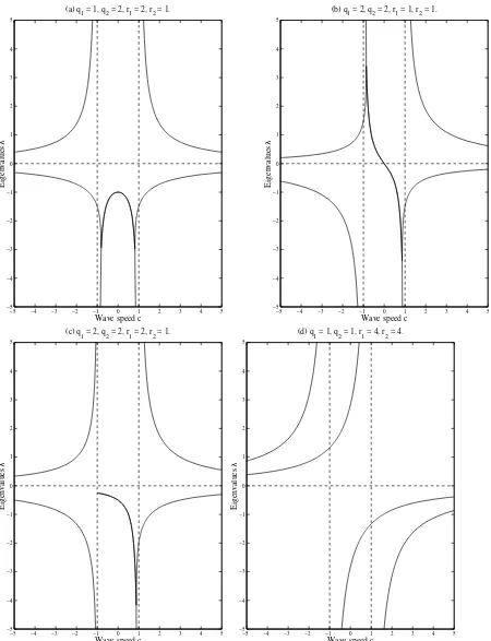
Figure 1: Bifurcation diagrams — plots of the eigenvaluesλ+ andλ−, ofK
c,θ(T), againstc (where the
−5 −4 −3 −2 −1 0 1 2 3 4 5 −5
−4 −3 −2 −1 0 1 2 3 4 5
(a) q
1 = 2, q2 = 2, r1 = 4, r2 = 4.
Wave speed c
Eigenvalues
λ
−5 −4 −3 −2 −1 0 1 2 3 4 5
−5 −4 −3 −2 −1 0 1 2 3 4 5
(b) q
1 = 1, q2 = 2, r1 = 2, r2 = 3.
Wave speed c
Eigenvalues
λ
−5 −4 −3 −2 −1 0 1 2 3 4 5
−5 −4 −3 −2 −1 0 1 2 3 4 5
(c) q
1 = 2, q2 = 1, r1 = 2, r2 = 1.
Wave speed c
Eigenvalues
λ
−5 −4 −3 −2 −1 0 1 2 3 4 5
−5 −4 −3 −2 −1 0 1 2 3 4 5
(d) q
1 = 2, q2 = 1, r1 = 1, r2 = 2.
Wave speed c
Eigenvalues
[image:17.612.74.524.89.678.2]λ
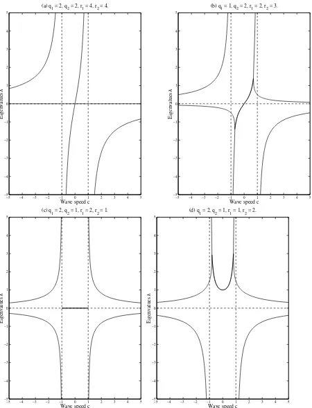
Figure 2: Bifurcation diagrams — plots of the eigenvaluesλ+ andλ−, ofK
c,θ(T), againstc (where the
Forc >−b2, note thatλ− is a stable monotone eigenvalue andλ+ is not, sincev+ <0 (asλ+ >θq1−r1
b1+c
in this case). Forc <−b1, note that neither eigenvalue is stable monotone asv− <0 andλ+>0. Thus, if there is a critical valuec(θ) it lies in the interval claimed. For b1=b2=b, say, this is enough to prove the lemma,c(θ) =−b, independent ofθ.
So, to complete the proof of the lemma it is sufficient to consider the caseb1> b2, where it is necessary to examine the eigenvalues when−b1< c <−b2, i.e. (b1+c)>0>(b2+c).
Examining the term under the square root in equation (16) (which we will denote byh(c), for fixedθ), for−b1< c <−b2, note that it can have one, two or no zeroes. If there are two zeroes let us denote them byc1 andc2, with−b1< c1< c2<−b2. Whenθq2> r2 andθq16=r1, there are two zeroes of hand for c1 < c < c2, h(c)<0. So in this case the eigenvalues ofKc,θ(T) are complex. When −b1 < c < c1 and whenc2< c <−b2,h(c)>0, so the eigenvalues are real. Whenc2< c <−b2 both eigenvalues are stable monotone. When −b1 < c < c1 the eigenvalues are not stable monotone — θq1 < r1 implies that the eigenvectors have components of opposite signs (as shown in Figure 1 (a)) while θq1 > r1 implies that the eigenvalues are positive (as shown in Figure 1 (b)). Thus, in this case,c(θ) =c2.
When θq2 > r2 and θq1 = r1 there is a single zero of h, at c1 say (as shown in Figure 1 (c)). When c1< c <−b2,h(c)>0 and both eigenvalues are stable monotone. When−b1< c < c1, h(c)<0 and so the eigenvalues are complex. Hencec(θ) =c1in this case.
Whenθq2 ≤r2 matters are simpler because θq1 < r1 implies that the eigenvectors have components of opposite signs or the eigenvalues are complex, within the interval−b1< c <−b2 (as shown in Figures 1 (d) and 2 (a) and (b)), andθq1≥r1 implies that the eigenvalues have non-negative real part throughout the interval−b1< c <−b2(as shown in Figures 2 (c) and (d)). Thus, for θq2≤r2,c(θ) =−b2.
Hence the lemma is proven.
Whenc=c(θ) there is a repeated stable monotone eigenvalue, unlessc(θ) =−bi, in which case the point
is moot since the stability matrix does not exist, but the analysis can be completed by direct methods (see section 4.6).
For the probabilistic method we need to look at one of these special cases in more detail — the case where−b1< c(θ)<−b2 andc=−b2. Note that−b1< c(θ)<−b2if and only if r2< θq2.
Recall thatKc,θ(T) is defined by equation (4), thus an eigenvectorv (with corresponding eigenvalue λ)
ofKc,θ(T) will satisfy the equation
λ(B+cI)v+ (R+θQ)v= 0. (18)
For (B+cI) invertible, this relation is also true in the opposite direction — a non-trivial vectorv that satisfies equation (18) is an eigenvector of Kc,θ(T) with eigenvalue λ. However, for (B+cI) singular,
equation (18) can still have non-trivial solutions, in the case of interest it has one solution,
λ=−(r1−θq1)(r2−θq2)−θ
2q 1q2 (b1−b2)(r2−θq2)
<0,
withv=
1 v2
, where
v2= θq2 θq2−r2
>0.
Thus this solution (which is what we are really interested in, analysis of Kc,θ(T) is a short-cut, and
simplifies discussion by giving us a way of referring to eigenvalues and eigenvectors as those ofKc,θ(T))
can be thought of as a generalized stable monotone eigenvalue ofKc,θ(T) and we have proved that, for
c > c(θ) the matrixKc,θ(T) has at least one (possibly generalized) stable monotone eigenvalue.
formula, which is shown in section 5.2 to be entirely equivalent to the preceding characterization, makes it easy to observe thatc(θ) is decreasing asθincreases and that
c∗:= lim
θ→∞c(θ) =−
b1q2+b2q1 q1+q2
.
This limit will be discussed in section 5.2, for now note that the lower bound onc(θ) given by Lemma 3.1 can therefore be tightened toc∗.
It is also possible to arrive at this limit by further manipulatingh(c). Rearranging the equationh(c) = 0 to express it as a quadratic inc (where the coefficients are quadratic in the other parameters, including θ) enables us to consider the limit asθ→ ∞by picking out the terms of highest order (i.e. order two in θ) only. Simplifying this expression yields
θ2
c(θ)(q1+q2) + (b1q2+b2q1) 2
+ terms of lower order inθ= 0.
Thus theθ2 term is zero if, and only if,c=c∗.
Further explicit calculation on Kc,θ(S) and Kc,θ(T) allows us to summarize the locations (i.e. left- or
right-half plane) of the eigenvalues as follows:
• Forc >−b2: both eigenvalues ofKc,θ(S) are real and positive, the smaller is unstable monotone,
the larger not; Kc,θ(T)’s eigenvalues are both real, forθ < ρ1+1ρ2 both are negative, forθ= 1
ρ1+ρ2 one is zero and the other is negative and forθ > ρ1+1ρ2 one is positive and one is negative.
• Forc <−b1: both eigenvalues ofKc,θ(S) are real and negative, the eigenvalue closer to zero is stable
monotone, the other not; Kc,θ(T)’s eigenvalues are real and positive for θ < ρ1+1ρ2, for θ= ρ1+1ρ2
one is positive and the other is zero and forθ > 1
ρ1+ρ2 one is positive and one is negative.
• For −b1 < c < −b2: the eigenvalues of Kc,θ(S) are real and have opposite signs, one is stable
monotone, the other unstable monotone; for θ < 1
ρ1+ρ2, Kc,θ(T)’s eigenvalues are real and have opposite signs, details for largerθ depend on the relative sizes ofcandc(θ).
The following result is required in our proof ofL1 convergence ofZ
λ in Theorem 5.4.
Lemma 3.2 (i) Suppose that c > c(θ). Let λs(c)be the stable monotone eigenvalue ofKc,θ(T)(the one
nearer to 0 if there are two). From the definition of Kc,θ andλs(c)it is easily seen that −λs(c)c is the
Perron-Frobenius eigenvalue of(λs(c)B+θQ+R). For µ < λs(c), withµsufficiently close toλs(c),
ΛP F(µB+θQ+R) =−µc1(µ)for some c1(µ)< c.
(ii) Asc↓c(θ), we have
λs(c)−1ΛP F(λs(c)B+θQ+R)→ −c(θ) and
∂
∂µΛP F(µB+θQ+R)
µ=λs(c)
→ −c(θ).
(iii) Whenc(θ)<−b2,Kc(θ),θ(T)has a double eigenvalue, which we will denote byλ0. This eigenvalue is
geometrically simple, i.e. it has only one normalised eigenvector even though it has algebraic multiplicity two, and is stable monotone.
Proof. We follow the proof of Lemma 4.4 of Crooks [6].
and λ0< µ < λs(c), there exists some c1(µ) such that c(θ) < c1(µ) < c and λs c1(µ) = µ and thus
ΛP F(µB+θQ+R) =−µc1(µ).
(ii) The first part follows from the fact that λs(c)−1ΛP F(λs(c)B +θQ+R) = c. For the second part
consider again the explicit form of the Perron-Frobenius eigenvalue as a function ofµ:
ΛP F(µB+θQ+R) = 1
2 µ(b1+b2)−(θq1−r1)−(θq2−r2)
+ 1
2 s
µ(b1−b2)−(θq1−r1) + (θq2−r2) 2
+ 4θ2q 1q2.
It is clear, by continuity (considering ΛP F as a function ofµand noting that the term under the square
root is strictly positive), that
∂
∂µΛP F(µB+θQ+R)
µ=λs(c)
→
∂
∂µΛP F(µB+θQ+R)
µ=λ0 asc↓c(θ) becauseλs(c)→λ0 asc↓c(θ). Now
∂
∂µΛP F(µB+θQ+R) = ∂
∂µΛP F(µB+µc(θ)I+θQ+R)−c(θ). (19)
We claim that ΛP F(µB+µc(θ)I+θQ+R) must attain a local minimum atµ=λ0. Note that, for fixed
c > c(θ), sufficiently close toc(θ), there are two values ofµ such that ΛP F(µB+µcI+θQ+R) = 0,
these two values ofµare the two stable monotone eigenvalues ofKc,θ(T). We now use a convexity result
due to Cohen [4].
To be precise, Cohen’s result states that the Perron-Frobenius eigenvalue of a matrix M1+M2 is a convex function of M2, where M1 has positive elements off the main diagonal and M2 is a diagonal matrix (possibly 0). Thus, for µ between the two eigenvalues ΛP F(µB+µcI +θQ+R) < 0 (strict
inequality since there can be at most two zeroes — each is an eigenvalue of Kc,θ(T), a 2×2 matrix).
Thus, forc=c(θ), ΛP F(µB+µc(θ)I+θQ+R)>0 except atµ=λ0 where it is zero.
Thus the derivative on the right hand side of equation (19) is zero atµ=λ0and hence the proof of (ii) is complete.
(iii) Ascdecreases throughc(θ) the two stable monotone eigenvalues of Kc,θ coalesce and, at least forc
sufficiently close toc(θ), become a complex conjugate pair with negative real part. From equation (16), λ0 = 12
n
θq1−r1
b1+c(θ)+
θq2−r2
b2+c(θ) o
, and from equation (17), this corresponds to an eigenvector of the form
1 v0
, where
v0=
(θq1−r1)−λ0 b1+c(θ)
θq1 .
We can verify directly that λ0 and v0 as given above have the correct signs (negative and positive respectively) by using inequalities arising from the definition ofc(θ).
For the probabilistic proof of uniqueness, modulo translation, of monotone travelling waves fromStoT, the next lemma is important.
Lemma 3.3 Suppose that c > c(θ) and that Kc,θ(T) has two stable monotone eigenvalues. Let β be
the stable monotone eigenvalue further from 0. Then, forα > β with αsufficiently close toβ, the only non-negative2-vectorg such that
0≤ α(B+cI) +θQ+R g
Proof. Convexity of ΛP F(µ(B+cI) +θQ+R) as a function of µ given by Cohen’s Theorem [4], for
β < µ < λ, yields ΛP F(µ(B+cI) +θQ+R)≤0. However, there can only be two values (µ1 andµ2, say) ofµ at which this function is 0 since eachµi is thus an eigenvalue of a 2×2 matrix. These two values
are thereforeβ andλand the inequality is strict.
Suppose that for some µ satisfying β < µ < λ, there exists g, non-negative, with g 6= 0, and (µ(B+cI) +θQ+R)g >0.Then ΛP F(µ(B+cI) +θQ+R)≥0 which is a contradiction.
Finally, we need the following result in showing that
Px,y
Zλ(∞) = 0= 0 or 1.
Lemma 3.4 If wis a2-vector such that 0≤w≤1 and
R(w2) = (R−θQ)w,
then either w= (1,1)or w= (0,0).
Proof. Rearranging the above equation notice that the problem amounts to searching for intersections of two parabolae inside the unit square —θq1w2= (r1+θq1)w1−r1w21 andθq2w1= (r2+θq2)w2−r2w22. Since each parabola goes throughw = (0,0) and w = (1,1) there can be no other intersections in the square — since from (0,0) to (1,1) the curveθq1w2 = (r1+θq1)w1−r1w12 is above the linew2 =w1
while the other curve is below it.
4
Analytic proofs of existence and uniqueness of travelling
waves
4.1
Plan of attack
To prove Theorem 1.1 we use shooting arguments. First note that the path of any solutionwof (2) which satisfies
w(x)→T as x→ ∞, w(x)→S as x→ −∞ and w′(x)>0, x∈R, must lie entirely inside the open unit square. Whether it must also lie between the nullclinesw′
1= 0 and w′
2 = 0 depends on the values of various parameters, as explained below. Depending on the geometric configuration of the nullclines, we introduce shooting boxes. We observe that these regions have four key properties upon which our proof will be based:
• Non-constant solution curves do not intersect the boundary of the region tangentially and hence any non-constant solution curve which intersects the boundary crosses it transversally;
• Exit-times of solutions in the regions are continuous functions of initial conditions;
• No non-constant solution curve passes throughS or T;
• Other thanS andT there are no equilibria in the closure of these regions.
4.2
Labelling the phase plane
In the 2-dimensionalw= (w1, w2)-plane consider the parabolae
P1:θq1w2−(r1+θq1)w1+r1w12= 0
and
P2:θq2w1−(r2+θq2)w2+r2w22= 0
and let Ωi denote the open region in the first quadrant between Pi and the wi-axis, i= 1,2. The
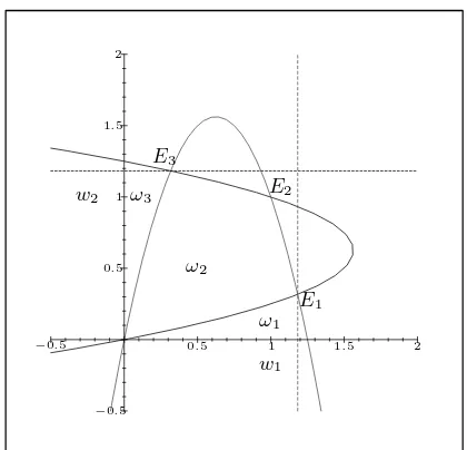
parabolae are of course the nullclines for the system, and their intersections are its equilibria. The point S = (0,0) ∈ P1∩P2 for all θ >0, the point T = (1,1) ∈ P1∩P2 for all θ > 0 and E± ∈ P1∩P2 if 0< θ≤(4ρ1ρ2)−
1 2.
Note that the relative positions of E+, E− and T depend on the value of θ and that no two of them
are commensurate with respect to the partial ordering onR
2 induced by the positive quadrant. Let us denote byE1the element of{E+, E−, T}with the largestw1-component and byE3 that with the largest w2-component. Then, forθ(ρ1+ρ2)<1,T =E2. Whenθ(ρ1+ρ2)>1 andθ≤(4ρ1ρ2)−
1
2,T could be E1 orE3. In this caseT =E1 forρ2> ρ1,T =E3forρ1> ρ2. The various equality cases missed out of this enumeration are those where equilibria coincide.
Also note that the relative position ofT and the maximum of the parabolaPi is determined by the sign
ofθqi−ri — ifθqi ≥ri then the segment ofPi from S to T is monotone; if θqi< ri then this segment
has a turning point before reachingT.
Regions of interest. Now let ˜Σ denote the rectangle in thew-plane with two sides on the axes intersecting at 0, a side throughE1 parallel to {w1 = 0} and one through E3 parallel to {w2 = 0}. Let Σ denote the open convex subset of ˜Σ whose boundary comprises four straight-line segments from∂Σ, a parabolic˜ segment fromP1joiningE1toE2and a parabolic segment fromP2joiningE2toE3. Thus the boundary of Σ always has four straight-line segments: in addition it has two parabolic components whenE+, E−
and T are distinct, one parabolic component when two of E+, E− and T coincide and no parabolic
component whenθ >(4ρ1ρ2)− 1
2. Also Σ consists of the union of three sets: ω
2= ˜Σ∩Ω1∩Ω2, a relatively closed component ω3 whose boundary intersects{w1= 0} away from the origin and a relatively closed componentω1whose boundary intersects{w2= 0} away from the origin. (See Figure 3.) Note that
(r1+θq1)w1−r1w21−θq1w2 >0, (w1, w2)∈ω2∪ω1, (r2+θq2)w2−r2w22−θq2w1 >0, (w1, w2)∈ω2∪ω3;
and hence, ifw= (w1, w2) satisfies (2) then,
(b1+c)w1′ is strictly positive atxifw(x)∈ω2∪ω1,
(b2+c)w2′ is strictly positive atxifw(x)∈ω2∪ω3, (20) (b1+c)w′1 is strictly negative atxifw(x)∈ω3\ω2,
(b2+c)w′2 is strictly negative atxifw(x)∈ω1\ω2.
A monotone curve connectingS to E1 must approachE1 from ω1∪ω2. Thus, by (20), if (b1+c)<0 there cannot be a monotone connection fromS to E1. Similarly, a monotone curve connectingS toE3 must approachE3 from ω2∪ω3. Thus, by (20), if (b2+c)<0 there cannot be a monotone connection fromS toE3.
A monotone connection toE2must eventually approach throughω2, so a necessary condition for existence is (b1+c)>0 and(b2+c)>0.
w1
w2
E1
E2
E3
ω1
ω2
ω3
−0.5
−0.5
0.5 0.5
1 1
1.5 1.5
[image:23.612.192.402.100.302.2]2 2
Figure 3: The regions of interest
square and must eventually approach T through some ωi. It is possible to work with just ω2 and ω3 — since ω1 is mapped toω3 by swappingb1 and b2, r1 and r2 and q1 and q2. (It is not possible for a monotone connection fromStoT to lie partly withinω1and partly withinω3since bothw′1andw′2have signs opposite inω1 to their signs inω3.) Theoutsideregion isω3 intersected with the unit square; the
insideregion is a subset ofω2inside the unit square. Examination of these two regions allows us to cover all possible monotone connections toT — connections must eventually approach from one of the two. Also note that the nullclines represent points at which solution curves are vertical or horizontal (where the nullclines cross, there are fixed points). Thus, if a solution curve hits a nullcline somewhere other than an equilibria it immediately crosses to the other side of the nullcline, tangency is not possible since the nullclines are nowhere vertical (for the one representing vertical solution curves) and nowhere horizontal (for the other).
4.3
The inside region
Consider the region formed by the segment of the parabolaP1 from S to the first intersection with the linew2= 1 (this is atT if θqr11 >1); if the intersection is not atT then use the linew2= 1 to connect the endpoint of the segment toT; the segment ofP2fromSto the first intersection with the linew1= 1 (this is atT if θq2
r2 >1) and if the intersection is not atT then use the linew1= 1 to connect the endpoint to T. Thus, theinside region is defined to be the regioninsideboth parabolae and the unit square, in the notation of the previous section it is a subset ofω2. See Figures 4 and 5.
Denote the edges of the region as follows:
• The open segment ofP1 (not includingS or the other endpoint) byA.
• The open segment ofP2 (not includingS or the other endpoint) byB.
w1
w2
−0.5
−0.5
0.5 0.5
1 1
1.5 1.5
2 2
A
B C
D x
y
S
[image:24.612.193.402.125.330.2]T
Figure 4: An example of an inside region with 4 distinct edges
w1
w2
−0.5
−0.5
0.5 0.5
1 1
1.5 1.5
2 2
A
B D
y
S
T
[image:24.612.193.402.442.651.2]• If B does not connect S to T then denote the open segment ofw1 = 1 (not including endpoints) byD.
Notice that a monotone connection fromS to T must approachT from inside this region if bothC and D exist. If either C or D does not exist then it is possible to reach T monotonically from outside the
inside region— then we must use the outsideregion as discussed below.
IfC exists, then denote its left endpoint byxand ifD exists then denote its lower endpoint by y. By (20) and the following discussion, a necessary condition for a monotone connection that eventually approachesT from the inside region is thatc >max(−b1,−b2), i.e.
b1+c >0 and b2+c >0, (C1)
sincew′
1>0 andw′2>0 (throughout the interior of the region) if and only if (C1) holds.
Lemma 4.1 Assume (C1) holds. Then a solution curve that hits the boundary of the inside region at any point other thanS or T immediately crosses the boundary.
Proof. Consider the various segments of the boundary. OnAand at the pointx, if it exists,w′
1= 0 and w′
2>0. Thus (using continuity and the fact that the slope of this boundary is bounded and positive, so the flow is not tangent to the boundary) ifw(t)∈Aorw(t) =xthen there exists anǫ >0 such that for s∈(t−ǫ, t), w(s) is inside the region and fors∈(t, t+ǫ), w(s) is outside the region.
Similarly forB and y—w′
2= 0 andw′1>0 so the same argument works. ForC, if it exists, note thatw′
1>0 andw′2>0 onC and again the solution curve crosses from inside to
outside automatically. Similarly forD, and the lemma is proved.
4.4
The outside region
We have observed that there are monotone curves fromS to T that do not intersect the inside region, except atT itself, when the inside region does not have four edges. Without loss of generality assume that the edgeCof the inside region does not exist, i.e.θq1
r1 >1, so that there is a possibility of a monotone connection throughω3. When neitherC norDexists there are two outside regions, by equation (20) the flow is in opposite directions in the two regions. Hence there can be a monotone connection through at most one of them.
Consider the region formed by the segment of the parabola P1 from S to T; the w2 axis and the line w2 =m(w1−1) + 1 for somem∈(0,1−θqr11). This restriction onm ensures that the line has positive slope and lies above the parabolaP1(the upper bound just given is the slope of the parabola atTand the assumption that θq1
r1 >1 ensures that the slope is strictly positive). We will choose a particular value of mlater. In the notation of section 4.2 this region is therefore a subset ofω3. See Figure 6 for a diagram of a typical example of this region.
Denote the edges of the region as follows:
• The open segment ofP1 (not includingS or T) byA.
• The half-open segment of thew2 axis (not includingS but including the other endpoint) byB.
• The open segment ofw2=m(w1−1) + 1 strictly between thew2 axis andT byC.
For a monotone connection fromS to T that does not go through the inside region it is necessary that w′
w1
w2
−0.5
−0.5
0.5 0.5
1 1
1.5 1.5
2 2
A B
C
S
[image:26.612.192.402.100.303.2]T
Figure 6: An example of an outside region
S to T that exit the outside region throughCand still converge monotonically toT this condition will still be necessary).
Using equation (20) to consider the direction of the flow within the region notice that is is therefore necessary that b2 > b1 and that −b2 < c < −b1, i.e. (b2+c) > 0 > (b1+c). So, for there to be a possibility of a monotone connection that is not through the inside region, the following conditions are necessary:
(b2+c)>0>(b1+c) and
θq1
r1 >1. (C2)
For a monotone connection through the other outside region it is necessary that (b1+c)>0>(b2+c)and
θq2
r2 >1 — the subsequent analysis is entirely equivalent since we can simply interchange the subscripts 1 and 2. The two cases are clearly mutually exclusive.
The condition (C2) ensures that, for eachk > 0, a curve that satisfies w′
2/w1′ =k is an ellipse passing throughS andT. This observation is used below to rule out internal tangencies to the region.
A solution curve cannot exit from the outside region throughA or B in forwards time. On A observe thatw′
1= 0 andw′2>0 and on B thatw′1>0 andw′2>0.
We need to check that the flow does not have an internal tangency toCin order to construct a shooting argument for the outside region. The shooting argument used runs backwards in time, but note that a tangency backwards in time is also a tangency forwards in time, and vice versa.
Lemma 4.2 Assume condition (C2) holds. Then a solution curve that hits the boundary of the outside region (from the inside of the region — an external tangency is immaterial) at any point other thanS or
T immediately crosses the boundary.
interior of the region — wherew′
1 >0 and w′2 >0 — and must eventually hit the line C again or else approachT. This is since it cannot leave the region throughA because w′
1 = 0, w′2 >0 there. Call the first point at which this occursx2.
Thus, the solution curve is a smooth curve fromx1tox2, both of which are on the linew2=m(w1−1)+1, therefore there is a pointx3on this curve at which the curve has slopem. However, the curve on which the slope of the flow ismis an ellipse; an ellipse that passes throughS,T andx1 — sox3cannot be on
this ellipse. This contradiction proves the result.
4.5
The shooting argument
To establish the main result (Theorem 1.1) we shall use the preceding observations in a shooting argument through the outside region (backwards in time), as well as a more standard forward time argument from S toT for the inside region. Note that a monotone travelling wave fromS toT is possible only ifT has stable monotone eigenvalues. A corresponding unstable direction atS is also necessary, but this always exists when a stable monotone eigenvalue atT exists. (See the discussion before Lemma 3.2 in section 3.) It is known so far that ifc >max(−b1,−b2) then a monotone connection can only exist through the inside region — we show below that in this case it does indeed exist and is unique. For c < min(−b1,−b2) there cannot be a monotone connection fromSto T and forcin between then there may or may not be a monotone connection (which necessarily lies entirely in an outside region) — the determining factor is whetherc is greater thanc(θ). When such a connection exists it is unique.
4.5.1 Through the inside region when (C1) holds
Consider the intersection of the inside region with the circle of radius ǫ, centred at the origin,S. This is a segment of a circle with 2 endpoints on the boundary of the inside region. w′
1 >0 andw′2 >0 are necessary for a monotone connection through the region (i.e. (b1+c)>0and(b2+c)>0 are necessary in this region) — when this is true a connection looks plausible. Considering the family of solution curves which pass through points of this segment at time zero completes our shooting argument, since, running backwards in time all these curves must go toS (since they cannot exit the region and cannot tend to any point other than an equilibrium), and running forwards in time, the curves from the 2 endpoints leave the region immediately and curves from points in between will exit transversally from the region (by Lemma 4.1), thus exiting in between the exit/end-points. Hence classical continuous dependence theory for initial value problems allows us the conclude that a monotone connection fromS to T exists.
4.5.2 Through the outside region when (C2) holds
Assume condition (C2), otherwise there is no monotone connection through the region. This time we shoot backwards in time.
Firstly we deal withc > c(θ). Choosemso that the edgeChas slope equal to half that of the dominant eigenvector ofKc,θ(T) (the dominant eigenvector is that corresponding to the negative real eigenvalue
of smallest modulus — when (C2) and c > c(θ) there are two simple stable monotone eigenvalues so m is well-defined). Thus the upper edge of the region bisects the angle between the line w2 = 1 and the dominant eigenvector atT. This enables us, backwards in time, to obtain paths leaving the outside region on both sides of T, and hence shoot to S. More precisely, for c > c(θ) we already know that Kc,θ(T) has two stable monotone eigenvalues. Consideration of equation (17) shows that both have slope
less than that of theP1 at T. The dominant eigenvector is
1 v+
. Thus we choosemto correspond
to a direction
1 v+/2
fact that the flow is determined by the dominant eigenvector we observe the flow sweeps through the boundaries of the region (by Lemma 4.2) as we follow a segment of a circle aroundT that intersects the region. Classical continuous dependence theory for initial value problems tells us that a connection from S toT exists.
Forc < c(θ) there is no stable monotone eigenvalue atT and there cannot be a monotone connection. Thus we have completed showing that a monotone eigenvalue at T is sufficient (except for the cases c = c(θ) and c = max(−b1,−b2) > c(θ) which are discussed below in section 4.6) for a monotone connection — we already knew it was necessary.
4.6
Special cases
We have been wary of the cases wherec =c(θ) andc =−bi. Assume, without loss of generality, that
b1> b2.
Ifθq2≤r2, thenc(θ) =−b2. Forc=c(θ) the only candidate for a connection fromStoT is the segment of thew2-nullcline,P2, connectingStoT. Ifθq2< r2then this is not monotone fromStoT and so there is no monotone travelling wave at this speed. Whenθq2=r2this connection is monotone. The travelling wave equations consists of one algebraic — defining the nullcline — and one differential equation. We can subst