www.elsevier.nl / locate / econbase
Welfare for the elderly: the effects of SSI on
pre-retirement labor supply
a ,* b
David Neumark , Elizabeth Powers
a
Department of Economics and NBER, Michigan State University, East Lansing, MI 48824, USA
b
Institute of Government and Public Affairs and Department of Economics, University of Illinois, Urbana, IL 61820, USA
Received 1 July 1998; received in revised form 1 November 1998; accepted 1 December 1998
Abstract
This paper studies pre-eligibility-age labor market disincentives created by the Supple-mental Security Income (SSI) program. Asset and income limits might induce individuals nearing the eligibility age to work less. We exploit states’ supplementation of federal SSI benefits to estimate the effects of SSI on pre-retirement labor supply, using SIPP data. We find some evidence that generous SSI benefits reduce the pre-retirement labor supply (and earnings) of men who are likely to participate in SSI after retirement, as they near the eligibility age, especially men who are eligible for early Social Security benefits, which may be used to offset their reduced labor income. 2000 Elsevier Science S.A. All rights reserved.
Keywords: SSI; Labor supply; Retirement
JEL classification: H31; J18; J14
1. Introduction
In recent years, the primary cash welfare program for families with children has been the object of intense scrutiny and debate, culminating in its radical overhaul in 1996. The case of this program, Aid to Families with Dependent Children
*Corresponding author. Tel.:11-517-353-7275; fax:11-517-432-1068. E-mail address: [email protected] (D. Neumark).
(AFDC), contrasts markedly with that of aid to the elderly poor provided through another welfare program, Supplemental Security Income (SSI), which has received
1
scant attention. A possible reason for this anomaly is that the public is more sanguine about how the contemporaneous work disincentives created by the existence of such a safety net affect the elderly, in contrast with younger groups such as families with children. However, little attention has been paid to the
pre-eligibility-age labor market disincentives created by such a program. In
particular, asset and income limits on eligibility for SSI might induce individuals nearing the eligibility age to reduce their labor supply. There is little if any hard evidence on such incentive effects, and this paper seeks to remedy this situation. There are two ways pre-eligibility-age work disincentives may arise due to the SSI program. Firstly, SSI’s income test discourages work prior to age 65. Since benefits are reduced or eliminated as post-retirement income increases, pension payments (including Social Security) reduce the potential SSI benefit. Some workers may have little incentive to continue working at older (pre-retirement) ages to increase private or public pension wealth further, as the extra post-retirement pension income crowds out SSI income. In addition, since SSI benefits are reduced or restricted on the basis of asset holdings at retirement through the asset test, the additional work needed to finance retirement savings is discouraged. Of course, the same sort of disincentive effects that affect labor supply may also affect saving, especially because of the asset test. In another paper (Neumark and Powers, 1998) we examine the effect of variation in SSI benefits on the saving of
2
those approaching the eligibility age. In this paper, we exploit the variation across states in supplementary SSI benefits to obtain difference-in-difference estimates of the effects of SSI on pre-retirement labor supply.
2. The incentive effects of SSI on pre-retirement labor supply
2.1. The SSI program
The SSI program was begun in 1974 to provide a uniform federal safety net for the elderly and disabled. This paper is concerned with the elderly component of the program, which sufficiently poor individuals may enter at age 65. The federal government sets eligibility criteria and maximum benefit levels for individuals and couples for the federal component of the program. In addition, some states (those with more generous safety nets prior to 1974) were required, and other states
1
SSI provides cash benefits to both the elderly and the disabled. In 1993 about 36% of those on SSI were enrolled in the program for the elderly. SSI and AFDC were comparable in terms of their total costs (between 25 and 26 billion dollars) (Blank, 1997).
2
chose to supplement the basic federal benefit. Federal benefits are indexed to inflation, while state benefits need not be. Benefits are reduced by income from other sources, including Social Security. Thus, other sources of retirement income influence both eligibility for SSI and the size of potential benefits. Financial resources also affect eligibility. For example, as of 1985 individuals with over $1600 in countable assets, and couples with over $2400 in countable assets, were
3
ineligible. In September 1984 (corresponding roughly to the time period covered by our earliest data) there were 1.55 million persons receiving SSI payments who
4
were eligible because of age (1995 Green Book). In 1991 (the period of our most recent data) 1.45 million aged persons received SSI (1994 Green Book, Table 6-1). As noted, some states supplement federal SSI benefits. If states choose to administer the SSI program, they are also free to set their own eligibility criteria such as asset limits. However, many states use the federal criteria, and they vary little in the other states (Social Security Administration, 1985). For example, in January 1985 the maximum federal benefit was $325 for an individual, and $488 for a couple. (Comparable figures for 1991 are $407 and $610.) The highest state benefit for couples was in California, which resulted in a maximum combined benefit of $504 for an individual, and $936 for a couple ($630 and $1167 for January 1991). In December 1985 the average federal benefit paid was $146 for individuals and $232 for couples, and the average state supplements were $97 and $257, respectively (Kahn, 1987), with 39% of SSI recipients receiving state supplements. In September 1989 the average federal payment to all elderly households on SSI was $162.84 and the average state supplement was $133.13; 49.6% of aged federal SSI recipients also received a state supplement (1990 Green
5 Book, p. 717).
The incentive effects of SSI on pre-retirement labor supply arise both because of a pure income effect of SSI benefits and because SSI benefits are reduced with other sources of income. Although other ‘post-retirement’ income reduces SSI benefits, the first $20 per month of unearned income (except means-tested transfer income), the first $65 of earned income, and one-half of earnings exceeding $65,
6
are disregarded in computing the SSI benefit. Therefore in states with no
3
Kahn (1987) discusses the definition of countable assets, and McGarry (1996) provides more details regarding the SSI program.
4
Zedlewski and Meyer (1989) estimate that in 1986 about 30% of the elderly poor received SSI benefits.
5
In 1993, 84.4% of benefits were paid for by the federal government, 13.3% of benefits were federally-administered state supplements, and the remaining 2.3% consisted of state-administered supplements (1994 Green Book, Table 6-1).
6
supplementation, or with supplementation but federal administration of the SSI program, monthly SSI benefits are determined by the formula
SSI5 G20.50hearned income2Minhearned income, $65j,0j 2hunearned income2Minhunearned income, $20j, 0j 2hmeans-tested transfer incomej,
where G is the guarantee, or the benefit paid when there is no other income. Earned income refers to the current (post-age-64) earnings of the SSI recipient. Unearned income includes income from private pensions, public pensions such as Social Security, interest income, and the like. Means-tested transfer income, such as Veteran’s Benefits, offsets SSI income dollar-for-dollar, and none of it is disregarded. The income disregards are not indexed for inflation, and did not vary over our sample period. They also are not differentiated by household type (couple or individual). For example, if both members of a couple each receive $200 per month in Social Security benefits, it is still the case that only $20 per month is disregarded from their total household unearned income for the purpose of computing their SSI benefit (1990 Green Book, p. 704, Table 3). In theory, then, 1984 SSI recipients could supplement their SSI-only incomes (from both earned and unearned income) by up to 26% for an individual and 17% for a couple before experiencing a decline in their SSI benefit (and by up to 21% and 14% in 1991). The law requires that SSI recipients apply for all other public benefits for which
7
they may be eligible. Consequently, in September 1989, for example, 70% of aged SSI recipients also received Social Security benefits; 18% also had some other unearned income, while only 1.7% reported any earned income (1990 Green Book, p. 732, Table 19). It is worth noting that only 41,005 SSI recipients reported income from a private employment pension at this time; this amounts to 2.8% of aged SSI recipients, although there may be some blind and disabled recipients included in this number (1990 Green Book, p. 733, Table 20). Presumably, this phenomenon is largely driven by the fact that SSI recipients are predominantly among the ‘permanently poor’ and have not been well-attached workers in the types of firms that would offer pensions as well as higher wages. Nonetheless, the relatively high percentages of SSI recipients receiving Social Security benefits and other unearned income suggest that the sort of disincentive effects on pre-retirement labor supply we discuss below are plausible.
2.2. Incentive effects
Considering the nature of the SSI benefit schedule, there are several situations that a pre-eligibility-age worker may find himself in with regard to current work
7
effort and future income. First, the typical household may be reasonably certain well before the head reaches age 65 that it will never be financially eligible for SSI. For example, in 1984, monthly ‘break even’ unearned incomes (i.e. the unearned income level at which benefits are reduced to zero) were $345 for an individual and $508 for a couple. If one could accurately determine the predetermined portion of post-eligibility-age unearned income (most importantly, future Social Security benefits), then households with future unearned income exceeding these break-even levels should not be influenced by the presence of the
8 SSI program and its rules.
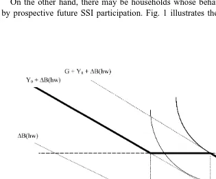
On the other hand, there may be households whose behavior could be affected by prospective future SSI participation. Fig. 1 illustrates the relationship between
Fig. 1. Trade-off between pre-retirement work effort and post-retirement unearned income with an SSI program.
8
current work hours and possible post-age-64 unearned income. Hours of work prior to age 65 are represented on the x-axis, while unearned income after age 64 for a retiree is represented on the y-axis. Y is the amount of unearned post-0
9
retirement income that is predetermined by past choices. G is the monthly SSI ‘guarantee’ (i.e. the benefit paid to an individual or couple with no other income). The function ‘DB(hw)’ relates current labor income (hours worked h times the
hourly wage w) to post-retirement, non-SSI income and is presumably increasing in its argument. This latter income may consist of Social Security benefits, private pension benefits, and the return on savings out of current earned income, although given the descriptive statistics cited earlier on the non-SSI income of aged SSI recipients, it is probably most realistic to think of this primarily as the incremental gain (in perpetuity) in Social Security benefits. In Fig. 1, the function ‘DB(hw)’ is
drawn as a line for ease of illustration.
For completeness, we assume that the predetermined portion of retirement income does not already exceed $20 per month. So long as the addition to future income from current work does not push unearned income above $20 per month, an additional hour worked today results in an increase in future unearned income of DB9(hw)w. As hours increase, the disregard level will be exactly met (at
BE 21
break-even hours H1 5 DB (202Y ) /w). Above these hours, increases in0 future unearned income due to increases in current labor supply will be exactly BE offset by decreased SSI benefits. Eventually, at break-even hours H2
21
(5 DB (201G2Y ) /w), the household obtains higher future income per hour0 worked today if they do not participate in the SSI program, but support themselves in retirement from income Y01 DB(hw). The effective budget constraint faced by
an agent intent on maximizing future consumption for given hours worked today is 10
therefore illustrated by the heavy shaded line.
Given this budget constraint, one would expect to observe a group of future SSI BE
recipients with an incentive to work between zero and H1 hours in order to increase their post-retirement income. A higher guarantee should reduce the labor supply of these individuals, since presumably the pure income effect from a larger guarantee leads them to take more current leisure. One might also expect to see
BE
SSI recipients clustered at H1 hours, since no additional post-age-64 consump-BE
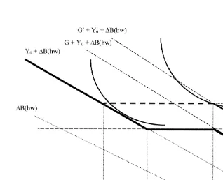
tion would be gained by working up to H2 hours. In this case, a ceteris paribus increase in ‘G’ widens the range of hours at which there is no future return to work, also reducing labor supply. The effect of an increase in G, and this latter labor supply effect, are illustrated in Fig. 2.
This simple analysis is contingent upon the assumption that future SSI recipients can reduce their labor hours prior to retirement and still maintain a satisfactory
9
Y can be thought of as a monthly annuity.0 10
Moffitt (1992) also discusses the phenomenon of ‘nonparticipating eligibles’ — those who locate
BE
Fig. 2. Optimal choice with lower (G) and higher (G9) guaranteed benefit.
level of current consumption. Relaxing this assumption weakens some of the predictions of the model. For example, we might observe potential SSI eligibles
BE BE
working between H1 and H2 hours prior to age 65, due to their current consumption needs, even though they gain nothing in terms of post-retirement consumption. However, the SSI benefit schedule would still bias against pre-eligibility-age labor supply, and the degree to which this effect is mitigated by pre-eligibility-age consumption needs can be treated as an empirical issue.
Social Security early retirement benefits are one alternative to labor income that could enable some 62–64-year-olds to reduce their labor market activity prior to
11
age 65 while maintaining consumption. For example, consider a person entitled to actuarially-reduced monthly benefits of $300 from the Social Security system at age 62 in 1985. This person could retire at age 62, receive $300 per month from
11
ages 62 through 64, and apply for SSI benefits at age 65. At 65 and thereafter, he would receive $300 monthly from Social Security and an additional $45 monthly federal SSI benefit. While pre-age-65 income may be lower than if the person had continued to work (because Social Security replacement rates are not 100%, even for extremely low-income workers, despite a progressive benefit formula), the disutility of labor counterbalances this.
In fact, individuals who may become eligible for SSI appear to have a stronger financial incentive than others to collect Social Security benefits prior to age 65. Normally, someone claiming Social Security benefits prior to age 65 faces a
permanent actuarial reduction in their benefit amount. For prospective SSI
recipients, however, Social Security’s actuarial reduction in benefits has no impact on their income after age 65, since the SSI benefit formula determines their net government transfer at the margin. For such individuals, the SSI program neutralizes the normal early retirement ‘penalty’. Because we are examining a very low-resource population that probably requires a continuing flow of income to support current consumption, Social Security early retirement appears to be a prime mechanism that would make reduced labor hours prior to SSI eligibility a desirable strategy. Therefore, when we examine the behavior of age groups nearing retirement in the analysis below, we explore the hypothesis that the effects of SSI are strongest for 62–64-year-olds, because we expect this group to have the best option to realize the incentive effects of the SSI program. (Of course, there may be other good reasons to take Social Security early retirement, such as ill
12 health, a possibility for which we allow in the empirical work.)
So far this discussion has ignored the asset test, which is an important feature of SSI and other welfare programs. As mentioned, ‘DB(hw)’ may be interpreted as
including asset income, and the arguments made above may be interpreted to mean that the value of working today to increase savings, and hence capital income tomorrow, is discouraged by the SSI benefit formula. The theory underlying the direct impact of asset tests on saving is described in Hubbard et al. (1995). Even modest financial savings will render a household ineligible for SSI by virtue of the asset test. Clearly, if asset tests discourage saving, then the presence of asset limits will also discourage the additional work needed to raise the stock of assets that would normally be drawn down during retirement. Moreover, assets that are drawn down in the run-up to eligibility for SSI (see Neumark and Powers, 1998) may
13
also be used to offset reduced labor income. The greater is the income floor provided by the welfare program, the more attractive it will be to choose a low-saving, distorted path of lifetime consumption, relative to a traditional smoothed life-cycle consumption path, and the more pronounced should be the disincentives for the additional pre-eligibility-age labor supply needed to finance life-cycle consumption.
12
We plan to examine more directly the interaction of Social Security and SSI in future work.
13
3. The data
Our household data are from the 1984, 1990, and 1991 panels of the Survey of 14
Income Program Participation (SIPP). As ultimately used, each single year of data provides a small number of observations on individuals from which the 15 effects of SSI are identified; consequently, we pool the data from all three panels. When weighted, samples of households drawn from the SIPP are nationally representative. The SIPP gathers detailed data on income and welfare program use that are impractical to collect in the larger Current Population Surveys. Each panel of households is interviewed every 4 months (each 4-month interval is referred to as a ‘wave’) for 2 to 3 years. Most questions are asked retrospectively about the previous 4 months. Corresponding to our earlier analyses with these data, we study labor supply measures in wave 4. We focus on samples of male heads of household
16 (including males living alone).
Our dependent variables are measures of labor market activity. We focus much of our attention on two standard labor supply measures: a binary employment variable that equals one if the individual reports positive hours of work in the first month of a wave; and actual hours of work in that month. In addition, we also examine results regarding the possible impact of the SSI program on monthly family earned income, for two reasons. First, family labor supply and the wages earned by each family member may influence post-retirement income and wealth, and work may be reallocated among family members so as to maintain current income but accumulate less post-retirement income. Second, family earnings (especially if there is only one worker) are a convenient ‘catch-all’ for the
14
When we began our initial work on the SSI program and saving behavior (Neumark and Powers, 1998), we used the 1984 panel because it is the largest sample by far (about one-third larger than the typical SIPP panel), and had the most thorough data on assets. When we began this paper, we expanded our data set to include the most recent panels then available in the interest of producing more up-to-date and more reliable estimates. At the time, the 1990 and 1991 panels were available on-line from the Census Bureau. (The Census Bureau puts out the panels from the intervening years on CD, but these do not contain the topical modules we need.)
15
We note, however, that the estimated effects of SSI on the labor supply measures can be rather variable across panels. In particular, for employment and hours the estimated effects are largest in the 1991 data and often near zero in the 1990 data, although the results for family earnings are stable. This suggests some caution in generalizing these results. It also suggests that we examine the validity of pooling the data across the 3 years. In results available upon request, we find that we do not reject the restriction of equal effects of SSI in the 3 years. Thus, strictly speaking, statistical tests allow us to pool the data, but we continue to urge some caution (and to anticipate analyzing other data sets) given the possible non-robustness of the results across the years.
16
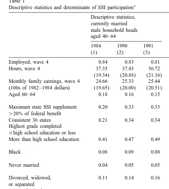
combined effects of changes in employment, changes in hours, changes in effort, etc., and as such may provide a bottom line for estimating the collective effects of SSI. In Table 1, columns (1)–(3) report descriptive statistics on these variables for the samples of men aged 40–64 for whom we estimate labor supply effects. Across the three surveys, 81 to 84% of the group is employed in wave 4, and
17
among workers, weekly hours average about 37. Average real monthly family earnings (in 1982–1984 dollars) are about $2500.
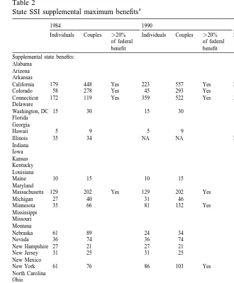
Each household is assigned a maximum state SSI benefit based on household composition (whether the household is comprised of an individual or a couple) and state of residence. Table 2 reports state supplemental (and federal) benefits as of January 1985, 1991, and 1992, which correspond approximately to the waves of the SIPP files that we use, taken from the 1994 and 1985 Green Books. We also show a classification of those states paying benefits exceeding 20% of the federal level, because in most of the empirical specifications we rely on a dummy variable indicating whether the state’s benefit (for either individuals or couples) exceeds this threshold; we do this to try to distinguish between states that have generous supplemental benefits, and states for which supplements are non-existent or
18
trivially small. However, we also examine results using alternative thresholds. Table 1 shows that 20% of our sample from the 1984 SIPP reside in states with state SSI supplements exceeding 20% of the federal benefit, with this percentage
19 rising to about 33% in the later panels.
Demographic variables in the analysis include race (black or non-black), marital status (married spouse present, never married, and ever married), and education (in a form described below). We use the overall unemployment rate in a state, taken from Employment and Earnings, to control for labor market conditions that might affect employment, hours, etc., as well as SSI participation. As explained below, we also require estimates of the probability of participation in SSI at or after age 65. We obtain these estimates by studying the determinants of SSI participation among those aged 65 or over. We use a dummy variable for SSI participation based on participation of the male at any time during wave 4.
17
Of course, business cycle conditions vary across these years, which we account for in the empirical estimation below.
18
There are some relatively minor additional complications with the benefits reported in the Green Book. See Neumark and Powers (1998) for further information.
19
Table 1
a
Descriptive statistics and determinants of SSI participation
Descriptive statistics, Probit for SSI
currently married participation, ever married male household heads male household
aged 40–64 heads aged 651
1984 1990 1991 Pooled SIPP panels
(1) (2) (3) (4)
Employed, wave 4 0.84 0.83 0.81
Hours, wave 4 37.35 37.43 36.72
(19.34) (20.88) (21.16) Monthly family earnings, wave 4 24.66 25.33 25.44 (100s of 1982–1984 dollars) (19.65) (20.00) (20.51)
Aged 60–64 0.18 0.16 0.15
Maximum state SSI supplement 0.20 0.33 0.33 0.016
.20% of federal benefit (0.003)
Consistent 36 states 0.21 0.34 0.34
Highest grade completed 20.005
3high school education or less (0.001)
More than high school education 0.41 0.47 0.49 20.073 (0.007)
Black 0.08 0.09 0.08 0.008
(0.004)
Never married 0.04 0.05 0.05 0.021
(0.005)
Divorced, widowed, 0.11 0.14 0.16 0.009
or separated (0.003)
Ever authorized 0.04 0.07 0.07 0.024
for food stamps (0.006)
State unemployment 7.57 5.49 6.71 0.003
rate (1.69) (0.88) (1.22) (0.001)
1990 20.003
(0.004)
1991 20.004
(0.003)
N 5016 5149 3459 5491
90th centile of predicted probability 0.043
a
Table 2
a
State SSI supplemental maximum benefits
1984 1990 1991
Individuals Couples .20% Individuals Couples .20% Individuals Couples .20%
of federal of federal of federal
benefit benefit benefit
Supplemental state benefits: Alabama
Arizona Arkansas
California 179 448 Yes 223 557 Yes 223 557 Yes
Colorado 58 278 Yes 45 293 Yes 56 323 Yes
Connecticut 172 119 Yes 359 522 Yes 325 461 Yes
Delaware
Washington, DC 15 30 15 30 15 30
Florida
Massachusetts 129 202 Yes 129 202 Yes 129 202 Yes
Michigan 27 40 31 46 14 21
Minnesota 35 66 81 132 Yes 81 129 Yes
Mississippi Missouri Montana
Nebraska 61 89 24 34 30 48
Nevada 36 74 36 74 36 74
New Hampshire 27 21 27 21 27 21
New Jersey 31 25 31 25 31 25
New Mexico
New York 61 76 86 103 Yes 86 103 Yes
North Carolina Ohio
Oklahoma 60 120 Yes 64 128 Yes 64 128 Yes
Oregon 2 2 2
Pennsylvania 32 49 32 49 32 49
Rhode Island 54 102 Yes 64 121 Yes 67 127 Yes
South Carolina Tennessee Texas
Utah 10 20 6 12 5 11
Virginia
Washington 38 37 28 22 28 22
West Virginia
Wisconsin 100 161 Yes 103 166 Yes 92 146 Yes
Maximum
federal benefits: 325 488 – 407 610 – 422 633 –
a
4. Empirical analysis and results
4.1. SSI participation
In our analysis, we exploit the state-level variation in SSI benefits to estimate the effects of SSI on labor supply. We do this via simple difference and difference-in-difference approaches that control for variation in labor supply behavior across states and across different types of individuals. We generically denote the labor supply measures we study as Y. Two factors influence the potential value of SSI benefits: the level of the benefits, and the likelihood of receiving them. Thus, for example, we might expect a person with characteristics associated with low permanent income (such as low education), in a state with high SSI benefits, to experience the greatest labor supply disincentives. In contrast, a white, married college graduate is extremely unlikely to be eligible for SSI, whether he resides in a state with high or low benefits. Thus, to estimate the effects of SSI, we focus on variation in labor supply behavior associated with high SSI benefits for those with a relatively high likelihood of eligibility.
We therefore begin by identifying exogenous characteristics associated with likely future SSI receipt, to characterize individuals as ‘likely participants’ or ‘unlikely participants’. By studying individuals over age 65, we can identify characteristics associated with a high likelihood of SSI participation. We then distinguish among workers under age 65 based on these characteristics, defining a dummy variable ‘Part’ to equal one for likely participants (based on a chosen threshold for the estimated probability of participating upon reaching age 65), and
20 zero otherwise.
Specifically, we estimate a probit model for the probability of participation among those aged 65 and over. These estimates — translated into derivatives of the probability of participation with respect to the independent variables — are reported for the pooled SIPP panels in column (4) of Table 1. In results not reported, we found evidence of a relatively strong non-linearity in the effect of schooling. In particular, up through a high school education, each additional year of schooling was significantly associated with a lower probability of SSI participation, but there was no effect of additional years of schooling (beyond high school). We therefore include in the specification reported here a dummy variable for more than a high school education, and an interaction between one minus this
21 dummy and years of schooling.
20
Because we assume financial resources are endogenous with SSI participation, we do not include them in our estimation of participation probabilities. Not surprisingly, financial resources are strongly negatively correlated with SSI participation (McGarry, 1996).
21
In addition to the effects of schooling, one would expect that more generous SSI benefits also increase the likelihood of participation; this is confirmed in the table, as the estimated coefficient on the dummy variable for generous state SSI
22 supplements (using the 20% threshold) is positive (0.016) and significant. To capture unobservables related to low permanent income, and possibly also unobserved heterogeneity in the propensity to participate in income-support 23 programs, information on food stamp enrollment is included in the probit. Information on whether an individual was ever authorized for food stamps is available in each panel, and is generally a significant positive predictor of SSI
24
participation. Finally, we also include the average state unemployment rate for the year, which is also significantly positively associated with SSI participation.
We use these probit estimates to generate predicted probabilities of participation in SSI for those aged 40–64. These in turn are used to construct the variable Part that is used in the labor supply equations. Although the supplement variable is included in the SSI probit, we do not use the variation in state supplements to construct Part. Therefore the observable characteristics of those classified as likely participants are the same in states with high and low SSI supplements, and the
25
same is true of those classified as unlikely participants. For most of the specifications we estimate, we define Part based on the 90th centile of the
22
We obtain the same result using a continuous measure of state supplements. Similarly, below we estimate models using different thresholds for defining ‘generous’ state supplements. A higher threshold always leads to a higher coefficient estimate for this variable.
23
This information comes from topical modules associated with different waves in the different SIPP panels. However, because this is a long-term measure, the timing should be inconsequential.
24
A referee suggests that because receipt of food stamps may be related to financial well-being, it may also be endogenous. Because this variable refers to whether one was ever authorized, rather than currently receiving food stamps, we suspect that this is not a problem. However, we also verified that the results were qualitatively similar when we excluded this food stamp variable from the SSI participation equation. Alternatively, since food stamp receipt probably does contain useful predictive information, we went in the other direction and substituted a dummy variable for current food stamp receipt, which should be more endogenous than ‘ever authorized’. With this variable substituted for whether one was ever authorized for food stamps, the estimated effects of SSI on labor supply were a bit weaker (but qualitatively similar) rather than stronger, implying that endogeneity of food stamp receipt does not bias the estimates in the direction of stronger effects of SSI on labor supply.
25
distribution of the predicted probabilities, but also report results with other thresholds; the 90th centile (0.043) is reported in the last row of Table 1. Based on a participation rate in SSI of 3.4% among those aged 65 and over in the SIPP files, a reasonable estimate is that about one-third of those above this centile would end up on SSI.
4.2. Alternative estimators of the effects of SSI on labor supply
We use the variable Part to divide the sample into likely and unlikely participants. We also use the state SSI supplement (initially) to divide states into those with generous supplements (i.e. greater than 20% of the federal benefit), and those with no supplements (denoting the dummy variable for the former as Supp), dropping the states with small supplements below the 20% threshold. We consider a number of simple difference, difference-in-difference, and difference-in-dif-ference-in-difference estimators. We explain each of these in turn, beginning with the simplest.
The effects of SSI are likely to be strongest for older workers who are nearing the age of eligibility, for two reasons. First, given stochastic influences on earnings and wealth, older workers can form better predictions of post-retirement income. Second, we suspect that workers pay more attention to the potential receipt of SSI benefits as they approach the age of eligibility. Consequently, we focus attention on workers nearest the age of eligibility. To begin, we define this group as 60–64-year-olds. Subsequently, we focus attention on 62–64-year-olds for whom, as discussed in the theory section, the effects of SSI benefits are likely to be strongest, as they can claim early Social Security benefits to maintain consumption
26
while reducing labor supply. For clarity, though, we explain our estimators in this subsection using ‘60–64-year-olds’ to indicate the older workers for whom we are estimating the effects of SSI.
We first estimate a simple difference (SD) estimator for the sample of likely participants aged 60–64, using the regression
Y5z 1 a ?Supp1Xc 1 e, (1)
where Y is the dependent variable related to labor supply, X is a vector of control variables, z is a constant, and e is a random error. a simply measures the difference between the behavior of likely participants in states with generous supplements, versus likely participants in states without generous supplements.
The simple difference estimated for 60–64-year-olds may yield a biased estimate of the effect of SSI if there are differences in labor supply behavior across states, perhaps attributable to differences in taxes, other policies, or preferences.
26
One possibility is that there are such differences, but that they are common to likely SSI participants of a wider age range in a state. Under this assumption, a solution to this problem is to study changes in behavior as likely participants approach the age of eligibility. Longitudinal data would provide a natural approach for this, but the SIPP panels are short (the 1990 and 1991 panels are only 2 years long). Instead, to study changes in behavior over time we rely on cross-cohort variation, examining differences in behavior between 40–59-year-olds and
60–64-27
year-olds. Letting Age6064 be the dummy variable indicating those in the 60–64 age range, we now use the sample of 40–64-year-old likely participants and estimate the difference-in-difference (DD) regression
Y5z 1 a ?Supp?Age60641b ?Supp1g ?Age60641Xc 1 e. (2)
In this regression b picks up the difference in Y, assumed common to all ages, between states with and without generous SSI supplements. g captures the difference in Y, common to all states, between 40–59 and 60–64-year-olds. Finally, a now captures the extent to which the difference in Y between 40–59 and 60–64-year-olds differs in states with generous SSI supplements, relative to states without generous supplements. Thus, this estimator of the effect of SSI nets out differences in the levels of Y between likely participants of all ages in the two types of states, and identifies the effect of SSI from the extent to which the difference in Y for likely participants in high-supplement states versus low-supplement states is greater (or less) for 60–64-year-olds than for 40–59-year-olds. This estimator uses the 40–59-year-old likely participants as a ‘control sample’ to capture state-specific differences that are common to all (40–59- and year-old) likely participants in a state. The ‘treatment sample’ consists of 60–64-year-old likely participants, with the ‘treatment group’ being those individuals in the treatment sample residing in states with generous SSI supplements. (The ‘control group’ is those individuals in the treatment sample with Supp equal to zero.) The key identifying assumption is that 40–59-year-old likely participants are not affected by SSI supplements but are influenced by other factors that might also generate differences in labor supply among 60–64-year-old likely participants between high- and low-supplement states. In other words, differences across states in the control sample capture differences between the treatment (high supplement) and control (low supplement) groups in the treatment sample that are not in fact due to the treatment of higher SSI supplements. In principle, we could use the alternative approach of exploiting variation over time in state supplemental benefits to estimate a model with fixed state effects. However, as shown in Table
27
2, variation over time in state supplements is minimal, with many states staying fixed (nominally) from year to year, and most states having only small changes over longer periods. Eq. (2) can be interpreted as using the relationship between Y and Supp for 40–59-year-olds to net out state-specific differences in Y that are correlated with, but not caused by, variation in SSI benefits, much as fixed state effects would do.
The motivation for the DD estimator in Eq. (2) was that the labor supply of likely participants may differ across states for reasons unrelated to SSI supple-ments; the assumption underlying Eq. (2) was that unobservables affecting labor supply were common to all likely participants (aged 40–64) in a state. An alternative assumption is that state-specific differences are common to all 60–64-year-olds in a state. In this case, we might consider only 60–64-60–64-year-olds, but compare the behavior of likely and unlikely participants. We would then use the DD estimator from the regression
Y5z 1 a ?Supp?Part1b ?Supp1g ?Part1Xc 1 e (3)
to estimate the effect of SSI. b again picks up the difference in Y between states with and without generous SSI supplements, although now the difference common to likely and unlikely participants aged 60–64, rather than the difference common to all likely participants aged 40–64.gcaptures the difference in Y, common to all states, between likely participants and unlikely participants. Finally,acaptures the extent to which the difference in Y between likely and unlikely participants differs in states with generous SSI supplements, relative to states without generous supplements. Consequently, this estimator of the effect of SSI nets out differences in the levels of Y between 60–64-year-olds in the two types of states, and identifies the effect of SSI from the extent to which the difference in Y in high-supplement versus low-supplement states is greater (or less) for likely participants relative to unlikely participants. Paralleling the earlier discussion of Eq. (2), this estimator uses the 60–64-year-old unlikely participants as a ‘control sample’ to capture state-specific differences that are common to all 60–64-year-olds (i.e. whether or not they are likely participants) in a state.
state. In this case, we use the sample of all 40–64-year-olds, and estimate the effect of SSI from the regression
Y5z 1 a ?Supp?Part?Age60641b ?Supp1g ?Age60641d ?Part (4)
1u ?Supp?Age60641k ?Supp?Part1l ?Age6064?Part1Xc 1 e.
In this regression b again picks up the difference in Y between states with and without generous SSI supplements,g captures the difference between 60–64- and 40–59-year-olds, and d measures the difference between likely and unlikely participants. The simple interactions capture the differences between older and younger individuals in high- vs. low-supplement states (u), likely and unlikely participants in high- vs. low-supplement states (k), and 60–64-year-old likely participants vs. unlikely participants (l). What a identifies, then, is the extent to which the difference in Y between 60–64-year-old and 40–59-year-old likely participants, relative to the difference between 60–64-year-old and 40–59-year-old unlikely participants, varies between high- and low-supplement states.
Alternatively, we can motivate this estimator by beginning with Eq. (3). This identifies the effect of SSI from the extent to which the difference in Y in high-supplement versus low-supplement states is greater (or less) for likely participants relative to unlikely participants. This could be inadequate if the difference in the overall level of labor supply between likely and unlikely participants differs in high- and low-supplement states for reasons other than SSI. In this case, we can assume that this difference is the same for 60–64- and 40–59-year-olds, and then use the 40–59-year-olds to obtain the same difference-in-difference-in-difference estimator. From this perspective, it is more intuitive to interpret the DDD estimatora as measuring the extent to which the difference in Y between 60–64-year-old likely and unlikely participants, relative to the difference between 40–59-year-old likely and unlikely participants, varies between high- and low-supplement states. Both interpretations of a in Eq. (4) are valid.
Although the DDD estimator is in a sense the most demanding, it is our preferred estimator because it controls for the most potential sources of bias. Nonetheless, at points throughout the paper we report the SD and DD estimates as well, in part to help reveal the effects of the alternative estimation methods.
One objection to the estimators in Eqs. (2) and (4) is that they infer changes in behavior from differences in behavior across cohorts that are very far apart. As an alternative, towards the end of the paper we examine some evidence from regressions in which we restrict attention to 60–64-year-olds, and use the difference between ages 60–61 and ages 62–64, in the same way as we use the difference between ages 40–59 and ages 60–64 (and ages 62–64) as described above. As noted above, rather than an arbitrary distinction, 62 is the age at which eligibility for early Social Security benefits is most likely to lead to a response to SSI.
differences in state supplementation of SSI to identify the effects of the policy. While the exploitation of state-level policy variation is a widely-used method to generate ‘quasi-experiments’, it is well known that if policy is itself endogenous, this approach does not necessarily produce unbiased estimates of the effects of exogenous policy variation (see Besley and Case (1994) for a discussion). A compelling assessment of the exogeneity of policy variation requires the spe-cification of instrumental variables for the policy, which we do not claim to have. However, in the present case we have good reason to believe that the policy variation reflects in large part long-term state differences, rather than short-term changes that might be partially in response to the dependent variables we study, which would be problematic. The reason for this is that much of the source of state-level variation in supplemental benefits reflects residual effects of earlier programs. As described in Kahn (1987), SSI was started in 1974 to replace state-administered income support programs to the elderly, blind, and disabled. Part of the state supplementation when SSI started was mandatory, because states were initially required to maintain the income levels of SSI recipients who had been supported by state programs prior to that year. Although states have adjusted benefits since then, in general there has been a great deal of persistence in the generosity of state supplementation. Thus, while we are not claiming that variation in SSI supplements is purely exogenous, we do not think it is driven much by responses to the behavior we are trying to capture in our dependent variables. Nonetheless, we acknowledge that state policies could in principle be related to relatively permanent differences across states in labor market conditions for older workers, in which case the DDD estimator would not necessarily identify the effects of SSI on these workers.
4.3. Basic results
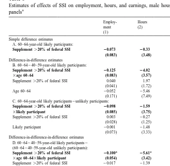
Table 3 reports the basic results for employment, hours, and family earnings. A probit is used for employment, an OLS regression for hours, and a one-tailed Tobit
28
for earnings. Table 3 reports the various simple difference (SD), difference-in-difference (DD), and difference-in-difference-in-difference-in-difference-in-difference-in-difference (DDD) estimates of the effects of SSI. In column (1), the estimated effects on employment are reported. Each of the estimates of the effect of SSI on the employment probability of 60–64-year-olds is negative. The SD, DD, and DDD estimates are in a fairly tight range (20.073 to 20.125). The DDD estimate is statistically significant at the 10% level; the point estimate, which we regard as the preferred estimate, implies that generous SSI supplements reduce the probability that likely participants aged 60–64 are employed by 0.10.
Column (2) turns to weekly hours of work, with very similar results. All of the estimators point to negative effects on hours of work of 60–64-year-old likely participants, although the range of estimates is larger, and again the estimate is statistically significant at the 10% level only for the DDD estimator. This latter estimate implies that generous SSI supplements reduce the weekly hours of likely participants aged 60–64 by about 5.6 hours.
Finally, column (3) reports the same analysis for family earnings. Strictly speaking, of course, this is not a labor supply measure, since wages may be endogenous. But as we argued above, family earnings may provide useful information on the combined effects of labor supply and other changes induced by SSI. The point estimates from the DD and DDD estimators are in a tight range (20.437 to20.537). In panels B and D, using 40–59-year-olds as a control group, the estimates are statistically significant at either the 5% or 10% level. This evidence on family earnings indicates that the labor supply reductions induced by SSI are for the most part not mitigated by changes in earnings among other family members, which is not surprising given the low labor force attachment of the
29 women in these cohorts.
Overall, we read the evidence to this point as providing some support for the hypothesis that more generous SSI benefits reduce labor supply of individuals approaching the age of eligibility who are relatively likely to participate in the program. For all three dependent variables, the DDD estimates indicate that generous SSI benefits reduce labor supply, with the estimated effects significant at
28
Although the hours are censored, the distribution of the uncensored data is far from normal, with large spikes at common values (such as 40). Thus, we use OLS to avoid inconsistent estimates stemming from a non-normal distribution. On the other hand, the uncensored log earnings observations appear approximately normal.
29
Table 3
Estimates of effects of SSI on employment, hours, and earnings, male household heads, pooled SIPP
a
Supplement.20% of federal SSI 20.073 20.33 20.088 220
(0.083) (3.48) (0.376)
Difference-in-difference estimates
B. 60–64240–59-year-old likely participants:
Supplement.20% of federal SSI 20.125 24.02 20.493* 1031 3age 60–64 (0.083) (3.57) (0.298)
Supplement.20% of federal SSI 0.040 1.97 0.263 (0.041) (1.72) (0.134)
Age 60–64 20.052 25.46 0.293
(0.171) (7.49) (0.611) C. 60–64-year-old likely participants2unlikely participants:
Supplement.20% of federal SSI 20.098 21.59 20.437 1632 3likely participant (0.085) (3.75) (0.353)
Supplement.20% of federal SSI 0.003 20.27 0.144 (0.028) (1.25) (0.109) Likely participant 20.001 21.48 20.388
(0.073) (3.33) (0.301) Difference-in-difference-in-difference estimates
D. 60–64240–59-year-old likely participants2
(60–64240–59-year-old unlikely participants):
Supplement.20% of federal SSI 20.100* 25.61* 20.537** 10,095 3age 60–643likely participant (0.054) (3.42) (0.241)
Supplement.20% of federal SSI 20.017 21.39 0.106 (0.009) (0.44) (0.029)
Age 60–64 20.207 215.98 20.593
(0.040) (2.43) (0.164) Likely participant 20.006 21.02 20.170
(0.023) (1.37) (0.091) Supplement.20% of federal SSI 0.015 0.78 0.017
3age 60–64 (0.018) (1.11) (0.074)
Supplement.20% of federal SSI 0.039 3.23 0.124
3likely participant (0.026) (1.57) (0.105) Age 60–643likely participant 0.019 0.20 20.144
(0.044) (2.86) (0.196)
a
the 5% or 10% level. This is the effect predicted by theory, as outlined in Section 2.
4.4. Specification analysis
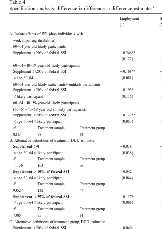
In this subsection we explore the sensitivity of our results to a number of choices regarding the definition of the sample and the empirical specification. We begin by excluding from the sample those individuals with a self-reported work-impairing disability. We do this to avoid the confounding influences of other income-support policies that also vary by state. Generally, states with high SSI supplements also offer relatively generous benefits in other transfer programs (this is necessarily true regarding SSI for the disabled). These programs may be available not only to those eligible for SSI for the aged, but also to younger men. To better isolate the incentive effects of SSI for the aged, therefore, we exclude individuals who report a disability that impairs their ability to work, since this may make them eligible for SSI for the disabled or other programs.
The estimates are reported in panel A of Table 4, for the SD, DD, and DDD estimators. Compared with the estimates in Table 3, for employment, hours, and family earnings the estimated effects of SSI are stronger when the work-impaired disabled are excluded; for all three dependent variables, the DDD estimates of the effects of SSI are statistically significant at the 5% or 10% level. Moreover, the results for the other estimators are very similar, with tight ranges of estimates, and, at least for employment and earnings, effects that are statistically significant at the 5% or 10% level. The point estimate of the effect on family earnings is probably implausibly large (recall that the dependent variable is in logarithms), but the estimate also has a relatively large standard error. The panel also reports the number of observations in the treatment sample and the treatment group. Note that the restriction to those without disabilities leaves us with a small treatment group, so neither the imprecision of the estimate, nor the likelihood of obtaining an
30
extreme value, is surprising. Nonetheless, the evidence of negative effects of SSI appears robust.
The similarity of the SD, DD, and DDD point estimates — once we remove the potential misspecification from including the disabled — is reassuring. In principle, the effects estimated by the DD or the DDD estimator may or may not stem largely from differences between the treatment and control groups in the treatment sample (the ‘main effects’). Although, conditional on the assumptions, the estimates are valid in either case, it is natural to place more confidence in the results if they show up in the main effects and are not driven primarily by differences in behavior among younger individuals or unlikely participants in high-and low-supplement states.
30
Table 4
a
Specification analysis, difference-in-difference-in-difference estimates
Employment Hours Log earnings
(1) (2) (3)
A. Isolate effects of SSI (drop individuals with work-impairing disabilities)
60–64-year-old likely participants:
Supplement.20% of federal SSI 20.246** 27.06 20.885* (0.122) (5.85) (0.452) 60–64240–59-year-old likely participants:
Supplement.20% of federal SSI 20.161** 26.68 21.026**
3age 60–64 (0.081) (4.76) (0.332)
60–64-year-old likely participants2unlikely participants:
Supplement.20% of federal SSI 20.193* 24.32 21.229**
3likely participant (0.115) (5.81) (0.497)
60–64240–59-year-old likely participants2
(60–64240–59-year-old unlikely participants):
Supplement.20% of federal SSI 20.127** 28.73* 21.129**
3age 60–643likely participant (0.053) (4.57) (0.306) N Treatment sample Treatment group
8243 98 18
B. Alternative definitions of treatment, DDD estimator
Supplement.0 20.038 22.49 0.053
3age 60–643likely participant (0.038) (3.13) (0.203) N Treatment sample Treatment group
11136 163 76
Supplement.10% of federal SSI 20.042 20.53 20.221
3age 60–643likely participant (0.044) (3.56) (0.233) N Treatment sample Treatment group
9352 132 47
Supplement.25% of federal SSI 20.117* 25.48 20.866**
3age 60–643likely participant (0.061) (5.15) (0.339) N Treatment sample Treatment group
7305 95 14
C. Alternative definitions of treatment group, DDD estimator
Supplement.20% of federal SSI 20.040 24.45* 20.346**
3age 60–643likely participant (70th centile) (0.032) (2.66) (0.172) N Treatment sample Treatment group
8243 322 81
Supplement.20% of federal SSI 20.066* 24.52 20.392*
3age 60–643likely participant (80th centile) (0.037) (3.15) (0.205) N Treatment sample Treatment group
8243 208 49
Supplement.20% of federal SSI 0.016 9.64 20.387
3age 60–643likely participant (95th centile) (0.074) (6.27) (0.412) N Treatment sample Treatment group
8243 52 9
a
Next, we turn to issues regarding the definition of the treatment (i.e. the definition of ‘Supp’), as well as the treatment group (i.e. the definition of ‘Part’). We continue to omit those with work-impairing disabilities, accepting the cost of a smaller treatment sample and treatment group, while avoiding possible misspecifi-cation of the effects of SSI. (For some of the different specifimisspecifi-cations to which we now turn, we get larger treatment groups.) We also restrict our focus to the preferred DDD estimates, to focus on a manageable set of results.
To this point we have identified the effects of SSI from differences in behavior between likely participants in states with SSI supplements exceeding 20% of the federal benefit, and states with no supplemental benefits (sometimes relative to the difference between unlikely participants in the two types of states). We therefore first report estimates using thresholds of 0, 10%, and 25% instead of 20%, reestimating both the SSI participation probit and the labor supply equations with these different thresholds for defining the variable Supp. We would tend to expect stronger results with the higher threshold, and vice versa, because the value of the program is higher.
Panel B of Table 4 reports results using these alternative thresholds for defining ‘generous’ state SSI supplements. For the 0 and 10% thresholds the estimated effects continue to be negative (with one exception), but are smaller than the corresponding estimates in panel D of Table 3, and not statistically significant. Thus, looking at the combined evidence, for the most part through the 20% threshold the effects are stronger the higher is the threshold used for defining generous state SSI supplements; this is always true for employment and earnings, and sometimes true for hours. However, the same is not true for the estimates using the 25% threshold, which are very similar to the estimates obtained using the 31 20% threshold for employment and hours, and smaller for family earnings. Because the states assigned to the treatment group vary as the benefits threshold is changed, this latter result indicates that the findings may be somewhat sensitive to relatively minor changes in which states are included in the treatment group, suggesting some difficulties in distinguishing the effects of SSI from other state differences that influence the labor supply of older individuals who are likely SSI
32
participants. Of course, a similar problem plagues virtually any study that uses state-level policy variation. For the most part, though, the estimated effects of SSI are stronger the higher the threshold used for defining ‘generous’ state-level SSI
31
In a preliminary version of this paper, we also experimented with a continuous measure of SSI supplements, although we think this is more likely to introduce measurement error, as the exact level of benefits may vary depending on living arrangements, the age of the spouse (since couples with a spouse below the age of 65 are eligible only for the individual benefit), and because of some other variations in policies regarding SSI benefit levels by state. Nonetheless, using linear and quadratic supplement variables (including all the interactions with the supplement measure), this same non-linearity of the effect of SSI was apparent, with the effect first rising with the size of the supplement, and then falling at relatively high levels.
32
benefits. Of course another factor that changes as we vary the threshold is the size of the treatment group (and the treatment sample). The lower the threshold, of course, the larger the treatment group. Thus, as the estimates and figures reported in panel B indicate, there is a trade-off between obtaining a larger treatment group and focusing on a treatment group for which the effects are likely to be stronger. In addition to choosing the threshold to define generous state SSI supplements, we also used an arbitrary threshold in defining likely participants, based on the 90th centile of the distribution of predicted probabilities of participation in SSI. Therefore, in panel C of Table 4 we also report results with different thresholds. We might expect weaker results for less stringent definitions of likely participants, although this is not necessarily the case because those with a very high probability of participation may face the prospect of so little retirement income that the incentive effects of SSI are inoperative. For the 70th and 80th centiles (reported in panel C of Table 4) and the 90th centile (reported in panel D of Table 3), for employment, hours, and family earnings the estimates always indicate larger effects of SSI the larger the centile, and the estimates are less likely to be significant the lower the centile. On the other hand, even using the 70th and 80th centiles we obtain some statistically significant effects at the 5% or 10% level. The results using the 95th centile are based on a much smaller treatment group, and the standard errors are correspondingly quite a bit larger. The results using this centile generally indicate weaker effects (if any) for employment, hours, or family earnings. Nonetheless, for the most part the results in panel C, coupled with the earlier estimates in Table 3, are consistent with those more likely to participate in SSI responding more strongly to the disincentives for labor market activity that
33 SSI creates.
Overall, we read the results in Table 4 as confirming our basic results, although raising some caution flags. On the one hand, many of the results indicate that for a wide variety of choices regarding the thresholds for benefits and participation, the evidence indicates negative effects of SSI on pre-retirement labor supply. Furthermore, for the most part the estimated effects of SSI change as we would expect them to as we vary the sample, the threshold for defining generous benefits, or the threshold for defining likely participants. On the other hand, not all of the results go in the expected direction. Thus, while the evidence points to negative effects of SSI on labor supply, the inference may be fragile.
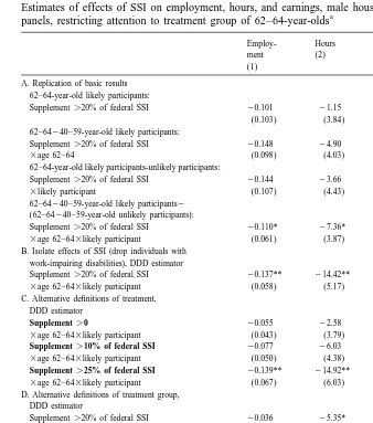
4.5. The effects of SSI at the age of eligibility for early Social Security benefits
The last set of analyses we report attempts to look at the data more finely to see whether pre-retirement labor supply effects of SSI are strongest once individuals reach the age of eligibility for early Social Security benefits. As explained in the
33
theory section, in this age range, but prior to eligibility for SSI (i.e. ages 62–64), individuals who expect to receive SSI at age 65 do not face the early retirement penalty encountered by other Social Security recipients. We explore evidence on this issue by repeating the earlier analysis, restricting the treatment sample and treatment group to 62–64-year-olds, instead of 60–64-year-olds as in the earlier tables. To keep the distinction between treatment and controls sharp, especially because 60 or 61-year-olds may begin to respond to the same incentives, we focus on specifications using ages 40–59 to define the control group for the DDD and one of the DD estimators.
The basic SD, DD, and DDD estimates are reported in panel A of Table 5. Compared with the same panels in Table 3, we find that for every estimator for each dependent variable, the estimated effects of SSI are larger for this more narrowly-defined age group. The remaining panels of Table 5 carry out spe-cification analyses similar to those described above. When we drop the work-impaired disabled, in panel B, the estimated effects of SSI become stronger, and are stronger than the corresponding estimates when ages 60–64 are used for the treatment group (panel A of Table 4). In panel C we vary the threshold for defining ‘generous’ state SSI benefits. The results are similar to those for the broader age group; in general the estimated effects are stronger and more likely to be significant the higher the threshold used, and the estimated effects are usually larger than we obtained looking at 60–64-year-olds. Similarly, in panel D we vary the treatment of the threshold for the predicted probability of SSI participation. We again generally find stronger estimated effects the higher the threshold, but here with thresholds of 70% and 80%, the effects are weaker than in Table 4, perhaps because the SSI–Social Security interaction only has a substantial effect for those
34
with a very high likelihood of eligibility for SSI. If one is relatively unlikely to take SSI, then Social Security early retirement is less attractive.
Finally, we turn to evidence on changes in behavior from ages 60–61 to ages 62–64. This is relevant for two reasons. First, as discussed above, we might expect the disincentive effects of SSI to become particularly strong beginning at age 62. While we have contrasted results for 60–64-year-olds and 62–64-year-olds, it is of interest to estimate more directly how behavior changes at age 62. Second, as noted earlier, much of our evidence of negative effects of SSI on labor supply is based on behavior of the DDD estimator that looks at comparisons relative to 40–59-year-olds. However, given the large span of years between the 60–64-year-old age group and the 40–59-year-60–64-year-old age group, cohort differences in labor supply could be influencing the estimates. By focusing attention on narrower cohorts that are much closer together, we should all but eliminate this problem.
These estimates are reported in panel E of Table 5. Not surprisingly, the
34
Table 5
Estimates of effects of SSI on employment, hours, and earnings, male household heads, pooled SIPP
a
panels, restricting attention to treatment group of 62–64-year-olds
Employ- Hours Log
Obser-ment (2) earnings vations
(1) (3) (4)
A. Replication of basic results 62–64-year-old likely participants:
Supplement.20% of federal SSI 20.101 21.15 20.180 138 (0.103) (3.84) (0.500)
62–64240–59-year-old likely participants:
Supplement.20% of federal SSI 20.148 24.90 20.552 949
3age 62–64 (0.098) (4.03) (0.343)
62–64-year-old likely participants-unlikely participants:
Supplement.20% of federal SSI 20.144 23.66 20.674 985
3likely participant (0.107) (4.43) (0.471) 62–64240–59-year-old likely participants2
(62–64240–59-year-old unlikely participants):
Supplement.20% of federal SSI 20.110* 27.36* 20.653** 9448
3age 62–643likely participant (0.061) (3.87) (0.275) B. Isolate effects of SSI (drop individuals with
work-impairing disabilities), DDD estimator
Supplement.20% of federal SSI 20.137** 214.42** 21.175** 7789
3age 62–643likely participant (0.058) (5.17) (0.353) C. Alternative definitions of treatment,
DDD estimator
Supplement.0 20.055 22.58 20.093 10,501
3age 62–643likely participant (0.043) (3.79) (0.248)
Supplement.10% of federal SSI 20.077 26.03 20.685** 8813
3age 62–643likely participant (0.050) (4.38) (0.293)
Supplement.25% of federal SSI 20.139** 214.92** 20.833** 6900
3age 62–643likely participant (0.067) (6.03) (0.403) D. Alternative definitions of treatment group,
DDD estimator
Supplement.20% of federal SSI 20.036 25.35* 20.223 7789
3age 62–643likely participant (70th centile) (0.036) (3.23) (0.210)
Supplement.20% of federal SSI 20.066 25.59 20.301 7789
3age 62–643likely participant (80th centile) (0.042) (3.75) (0.246) E. Closer cohorts, DDD estimator
62–6460–61yearold likely participants -(62–64-60–61-year-old unlikely participants), including work-impaired disabled:
Supplement.20% of federal SSI 20.140 210.52 20.690 1632
3age 62–643likely participant (0.184) (8.22) (0.757) Excluding work-impaired disabled:
Supplement.20% of federal SSI 20.425** 233.38** 20.977 1083
3age 62–643likely participant (0.181) (12.98) (1.074)
a
standard errors are relatively high because of the much smaller sample sizes relative to the DDD estimator using 40–59-year-olds. On the other hand, the point estimates indicate sizable changes in behavior for 62–64-year-olds relative to 60–61-year-olds. This is especially true when we omit the work-impaired disabled, although in this case the numbers of likely participants in the two age groups become very small, leading to large standard errors and perhaps to some implausibly large estimated effects. Overall, though, the evidence in Table 5 points to sharper disincentive effects of SSI on pre-retirement labor supply, and to rather marked changes in behavior beginning at age 62, although statistically this evidence is not always strong.
One interpretation of this set of findings is that offered in the theory section — namely, that the interaction of SSI and Social Security creates particularly strong labor supply disincentives in the 62–64 age range. An alternative interpretation, of course, is simply that as workers approach the age of eligibility for SSI, they are either more able to reduce their labor supply because their assets are sufficient to tide them over until they are eligible for SSI, or they become more responsive to the incentives posed by SSI as the age of eligibility looms closer. In principle, one might study this question by breaking up likely participants into single-year age groups and asking whether there is a discrete change in behavior at 62, or continuous change as individuals approach age 65, as well as by looking at receipt of early Social Security benefits. However, our treatment sample (60–64-year-old likely participants) is too small to engage in this sort of analysis. We therefore leave this question to future research, and plan to address it using the Health and Retirement Study when additional waves are available generating many observa-tions on individuals as they approach and pass the age of eligibility for SSI.
5. Conclusion
We use state-level variation in the generosity of supplemental SSI payments to identify the effects of SSI for the aged on labor supply as men approach the age of eligibility for the program, studying a sample of male household heads. We find some evidence that SSI discourages work among men nearing the age of eligibility, as predicted given the way the SSI program penalizes post-65 income and assets. We look at evidence on effects of SSI on employment, hours, and family earnings. Across different specifications, samples, and estimators, the point estimates of the effects of SSI are almost always negative, although the statistical significance of the evidence varies.
indicating that we are identifying real rather than spurious effects of SSI. In particular, we find that the estimated effects of SSI often vary as expected when we vary the level of benefits used to classify states as providing generous supplements, and when we vary the cut-off for identifying likely SSI participants. In our view, therefore, the evidence as a whole is most consistent with pre-retirement labor supply disincentives, although we repeat our caution emphasized in the paper that this inference is somewhat fragile.
Finally, as we would expect from the interaction of SSI with Social Security, we find that the effects are strongest among those aged 62–64. One intriguing interpretation of this finding is that the availability of SSI at age 65 encourages likely SSI participants to retire at age 62, financing this retirement out of early Social Security benefits. This has implications for how we might restructure SSI to avoid this added burden on the Social Security system. In particular, reduced SSI benefits for those who take early Social Security, paralleling the relationship between Social Security benefits and age of retirement, would be expected to discourage this type of behavior. More concrete evidence on the relationship between SSI and Social Security awaits further research.
This research also poses two further questions. First, can this finding be replicated in other data sets? It would be fruitful to explore similar evidence using other data sets. In particular, after more waves of the Health and Retirement Study are released, a large data set covering individuals right up to and past the age of eligibility for SSI will be available. We plan to analyze these data when they become available.
The second question concerns whether there are superior policies that avoid the disincentive effects of SSI. One possible mechanism for providing a minimum income floor for the elderly that has been broached in the context of the debate on Social Security reform is the ‘demogrant’ (Mitchell and Zeldes, 1996), which would provide a fixed, minimum guarantee to all of the elderly. Obviously such a program would be more expensive than SSI. But as part of a broader reform of Social Security the budget implications might be quite minimal, and it might successfully provide a minimum income floor while eliminating the disincentive effects of SSI on pre-retirement labor supply.
Acknowledgements