Received May 29, 2015Published as Economics Discussion Paper June 12, 2015
Revised July 16, 2016 Accepted September 29, 2016 Published October 10, 2016
Decision Making in Times of Knightian
Uncertainty: An Info-Gap Perspective
Yakov Ben-Haim and Maria Demertzis
Abstract
The distinction of risk vs uncertainty as made by Knight has important implications for policy selection. Assuming the former when the latter is relevant can lead to wrong decisions. With the aid of a stylized model that describes a bank’s decision on how to allocate loans, the authors discuss policy insights for decision making under Knightian uncertainty. They use the info-gap robust satisficing approach to derive a trade-off between confidence and performance (analogous to confidence intervals in the Bayesian approach but without assignment of probabilities). The authors show that this trade off can be interpreted as a cost of robustness. They show that the robustness analysis can lead to a reversal of policy preference from the putative optimum. The authors then compare this approach to the min-max method which is the other main non-probabilistic approach available in the literature. They also consider conceptual proxies for robustness and demonstrate their use in qualitative analysis of financial architecture and monetary policy.
(Published in Special Issue Radical Uncertainty and Its Implications for Economics)
JEL C02 C18 D81 G10
Keywords Uncertainty vs risk; confidence; robustness; satisficing; info-gap Authors
Yakov Ben-Haim, Yitzhak Moda’i Chair in Technology and Economics, Technion— Israel Institute of Technology, Haifa, 32000 Israel, [email protected]
Maria Demertzis, De Nederlandsche Bank, PO Box 98, 1000 AB Amsterdam, The Netherlands
1 Introduction
The economic circumstances since the start of the crisis in 2007 to the present are characterized by high levels of uncertainty. What do we mean by high uncertainty and what does it imply for policy design or decision making? High uncertainty can mean one of two things: either high stochastic volatility around known (or well estimated) average future outcomes, or at least partial ignorance about relevant mechanisms and potential outcomes. The first implies that uncertainty can be probabilistically measured (what Frank Knight called ‘risk’), whereas the second implies that it cannot (what Knight called ‘true uncertainty’ and is now known as Knightian uncertainty). We often conflate these two concepts when discussing ‘uncertainty’ in general. However, it is crucial to distinguish between them for three reasons. First, the relevant methods for decision making depend on which of the two notions of ‘high’ uncertainty we address. Designing policies under the assumption of probabilistically measurable risk can lead to serious policy mistakes if the underlying uncertainty is non-probabilistic, Knightian. Second, one’s measures of confidence differ under risk or Knightian uncertainty. Finally, the use of contextual understanding is different when dealing with risk or Knightian uncertainty. In a probabilistic setting contextual understanding can be used, for example, to select an appropriate probability distribution. In a Knightian setting contextual understanding can be used to intuit a trend or to sense a pending change that is not yet manifested in data.
This paper will make the following points:
• When uncertainty is probabilistically measurable risk, it is possible to design
policies that are optimal on average or in some quantile sense. Policy design under risk is based on first principles as expressed by economic theory. The theory underlies policy choices that are designed to optimize specified substantive outcomes (e.g. minimize a high quantile of the inflation, maximize average growth, etc.).
• Under Knightian uncertainty it is not possible to optimize stochastic
to prevent bad results from occurring or at least prepare for them. Building buffers in the financial system, applying unorthodox monetary policies in the monetary system are policies of this type; they aim to provide intervention tools to deal with or prevent bad outcomes from arising, irrespective of how likely they might be.
• A non-probabilistic concept of robustness is used to evaluate the confidence
in achieving an outcome under Knightian uncertainty. We will discuss info-gap robustness and compare it with the min-max robustness concept. We will illustrate both quantitative and qualitative implementations of info-gap robustness analysis for policy selection.
Decision making under risk relies on known probability distributions of out-comes. Policy design becomes a question of identifying the most likely occurrence (or perhaps a quantile of the occurrence) given the underlying models, and applying measures that optimize the outcome. Risks around those most likely occurrences are described probabilistically, and confidence in one’s actions is best captured with statistical intervals or similar probabilistic quantities.
However, probabilities are measures of frequencies of events that have hap-pened in the past, and therefore, in real time we are not necessarily confident that they represent accurate descriptions of the future. What does this mean for policy making? How can we evaluate confidence in these decisions? In this paper we provide an info-gap approach to decision making under Knightian uncertainty. With the aid of a simplified bank loan allocation example we will describe how the decision problem is handled in the presence of Knightian uncertainty. The info-gap approach will allow the bank to rank different portfolios in a way that it can pick those that provide satisfactory outcomes for the greatest range of adverse future contingencies. Robustness provides a measure of confidence.
for robustness and illustrates their use in qualitative policy analysis. Section 6 concludes.
2 Risk versus uncertainty: Implications for policy making
2.1 Risk versus uncertainty
Frank Knight (1921) distinguished between ‘risk’ (for which probability distribu-tions are known) and ‘true uncertainty’ (for which probability distribudistribu-tions are not known). Knightian uncertainty reflects ignorance of underlying processes, functional relationships, strategies or intentions of relevant actors, future events, inventions, discoveries, surprises and so on. Info-gap models of uncertainty pro-vide a non-probabilistic quantification of Knightian uncertainty (Ben-Haim, 2006, 2010). An info-gap is the disparity between what youdo knowand what youneed to knowin order to make a reliable or responsible decision. An info-gap is not ignoranceper se,but rather those aspects of one’s Knightian uncertainty that bear on a pending decision and the quality of its outcome.
Under risk we are confident—at least probabilistically—of the underlying model or combination of models that describe the economy. By contrast, under Knightian uncertainty, the social planner lacks important knowledge of how the system works. The planner starts with a number of models that may be relevant, but cannot identify the likelihood with which they describe the economy. When designing policy under risk, the knowledge of underlying probability distributions permits the identification of policies that are optimal on average or satisfy other quantile-optimality requirements. This is not possible under Knightian uncertainty because one lacks knowledge of the underlying distributions. But if one cannot design policy based on the principle of outcome-optimality, what other principles can one follow and what would these policies look like?
The literature on robust control relies on identifying and then ameliorating worst outcomes (Hansen et al. 2006, Sargent and Hansen 2008 and Williams 2007). The planner considers a family of possible models, without assigning probabilities to their occurrence. Then that model is identified which, if true, would result in a worse outcome than any other model in the family. Policy is designed to minimize this maximally bad outcome (hence ‘min-max’ is another name for this approach). In robust control one does not assess the confidence explicitly. Confidence manifests itself in the following form: the planner will have maximally ameliorated the worst that is thought to be possible. The optimization is not of the substantive outcome (growth, employment, etc.) but rather of ameliorating adversity. In this sense min-max is robust to uncertainty.
The appeal of min-max is that it provides insurance against the worst antic-ipated outcome. However, this technique has also been criticized for two main reasons. First, it may be unnecessarily costly to assume that the worst will happen (irrespective of how it is defined). Second, the worst may be expected to happen rarely and therefore it is an event that planners know the least about. It is not reliable (and perhaps even irresponsible) to pivot the policy analysis around an event that is the least known (Sims 2001).
The second approach is called info-gap (Ben-Haim 2006, 2010) and relies on the principle of robust satisficing.1 The principle of satisficing is one in which the
planner is not aiming at best outcomes. Instead of maximizing utility or minimizing worst outcomes, the planner aims to achieve an outcome that isgood enough. For example, the planner tries to assure that loss is not greater than an acceptable level, or growth is no less than a required level. When choosing between alternative policies, the robust-satisficing planner will choose the policy that will satisfy the critical requirement over the greatest spectrum of models.2
Info-gap theory has been used for a wide range of economic and policy plan-ning decisions. Zare et al. (2010), Kazemi et al. (2014) and Nojavan et al. (2016) study applications to energy economics. Chisholm and Wintle (2012) study
ecosys-1 The technical meaning of “satisficing” as “to satisfy a critical requirement” was introduced by
Herbert Simon (1955, 1957, 1997).
2 Satisficing is a strategy that seems to maximise the probability of survival of foraging animals in
tem service investments, while Hildebrandt and Knoke (2011) study investment decisions in the forest industry. Ben-Haim et al. (2013) employ info-gap tools in ecological economics. Yokomizo et al. (2012) apply info-gap theory to the economics of invasive species. Stranlund and Ben-Haim (2008) use info-gap ro-bustness to evaluate the economics of environmental regulation. Many further applications are found at info-gap.com
Min-max and info-gap methods are both designed to deal with Knightian uncertainty, but they do so in different ways. The min-max approach requires the planner to identify a bounded range of events and processes that could occur, acknowledging that likelihoods cannot be ascribed to these contingencies. The min-max approach is to choose the policy for which the contingency with the worst possible outcome is as benign as possible: ameliorate the worst case. The info-gap robust-satisficing approach requires the planner to think in terms of the worst consequence that can be tolerated, and to choose the policy whose outcome is no worse than this, over the widest possible range of contingencies. Both min-max and info-gap require a prior judgment by the planner: identify a worst model or contingency (min-max) or specify a worst tolerable outcome (info-gap).3 However, these prior judgments are different, and the corresponding policy selections may, or may not, agree.4
2.2 How do policies change as we account for uncertainty?
A vast literature has analyzed how policies designed to handle risk differ from those designed to handle Knightian uncertainty. In the case of designing policy under risk the most famous result is that of Brainard in his seminal paper (Brainard 1967) in which he showed that accounting for Bayesian uncertainty, in a specific class of problems, implies that policy will be more cautious.5 In terms of policy changes it therefore means smaller but possibly more persistent steps will be taken, and is known as the ‘Brainard attenuation’ effect. At the limit, as risk becomes
3 We will explain in detail later that usually the policy maker does not have to actually identify a
specific value for the worst acceptable outcome.
4 Further discussion of this comparison appears in Ben-Haim et al., 2009. See also Section 4 here.
5 This is for uncertainty in the coefficients that enter the model multiplicatively, not the residuals
very large, the social planner abandons the use of the instrument and is faced with policy inaction.6As the social planner is more and more uncertain of the results of policy, it is used less and less. This result has been very popular with policy makers as it appeals to their sense of caution when they lack sufficient information or knowledge.7
By contrast, policies derived under the principle of min-max (or robust control), and directed against non-probabilistic uncertainty, tend to be comparatively more aggressive. The policy steps taken are typically larger in size by comparison to either risk-based policies or outcome-optimal policies in the absence of uncertainty. The intuition is that under Knightian uncertainty, and when addressing a worst case, there is little knowledge about the transmission mechanisms, and it is therefore important to strongly exercise available tools in order to learn about and manage the economy. It is not surprising that this runs against some policy makers’ natural inclination to be cautious and avoid introducing volatility.
It is here that info-gap robust satisficing provides a useful operational alterna-tive. At the heart of the method for dealing with uncertainty lies a fundamental choice: that between robustness against uncertainty and aspiration for high-value outcomes. As we become more ambitious in our aspirations, we need to compro-mise in the degree of confidence that we can have about achieving these aspirations. Conversely, if we require high confidence in achieving specified goals, then we need to reduce our ambitions. Info-gap is a method developed with the specific aim of assessing this trade-off. Confidence is quantified with robustness to un-certainty. The trade-off quantifies the degree of robustness with which one can pursue specified outcome requirements. Policies therefore are not automatically more or less aggressive. It depends very much on the decision maker’s preferences. Furthermore, the decision maker can rank alternative policies: between policies of similar ambitions, those that provide the greater robustness (greater confidence) are preferred. In Section 4 we will compare and contrast the policy implications of min-max with robust-satisficing.
6 To be fair, this attenuation effect does not hold always but also depends on the cross-correlations
of error terms in the assumed model. It is possible therefore, that the policy is more aggressive than that under no uncertainty and Brainard did acknowledge that.
3 An informative trade-off: Robustness vs performance
In this section we use a highly simplified example to illustrate how a decision maker comes to informed decisions despite the inability to measure uncertainty. We provide a framework, based on info-gap theory, that allows us to derive a trade-off between confidence in outcomes and performance requirements. Decision makers who are ambitious in terms of requiring high-performance outcomes will have to settle for their choices being appropriate only across a small range of events or contingencies (i.e. having low robustness). On the other hand, if the decision maker wants the comfort of knowing that policies chosen will function across a wide range of contingencies (high robustness), then relatively low performance outcomes will have to be accepted. We also show that policy prioritization often does not require the choice of a specific outcome.
Consider a bank that aims to give out loans to potential borrowers. Part of the problem that it faces is that the premium it requires depends on the risk type of the recipient agents, where risk here refers to their likelihood to default. However, assessing this probability is subject to Knightian uncertainty and therefore the bank is not in the position to price risk based on well defined underlying distributions. Furthermore, correlations exist between the solvencies of different borrowers that are significant even when they are small. Inter-borrower correlations are typically assumed to be zero though this is quite uncertain, potentially leading to over-optimistic estimates of bank invulnerability (Ben-Haim, 2010, Section 4.1).
In evaluating or designing the bank’s loan portfolio, the following two questions (among others) are pertinent. First, some of the uncertainty in assessing default probabilities can be reduced. How much reduction in uncertainty is needed to substantially increase the bank’s confidence? How should uncertainty-reduction effort be allocated among different borrower profiles as characterized by their estimated default probabilities? Second, what loan-repayment programs should be used for clients with different default-probability profiles? We describe how info-gap can help banks to allocate loans and, in Section 4, we compare it with the robust control (min-max) approach.
3.1 Formulation
Consider a bank that plans a number of loans, all with the same duration to maturity. The potential borrowers are of different risk types but all borrowers of the same risk type are identical.
Let:
N: number of years to loan maturity
K: number or risk-types
fkn: repayment in yearnof risk typek
f: matrix of fknvalues
wk: number (or fraction) of loans of risk-typek
w: vector ofwkvalues
Nd: number of years at which default could occur
tj: year at which default could occur, for j=1, . . . ,Nd
pk j: probability that a client of risk-typekwill default at yeartj
p: matrix of default probabilitiespk j
i: discount rate on loans
In case of default attj, no payment is made in that year and in all subsequent
years, for j=1. . .Nd. We definetNd =N+1, so “default” at yeartNd means that
the loan is entirely repaid and default has not occurred. We also assume that
pk1. . .pkNd is a normalized probability distribution, so that the probability that
borrowers of risk-typekdo not default is:
pkNd =1−
Nd−1
∑
j=1pk j. (1)
The present worth (PW) of the entire loan portfolio, assuming no defaults, is:
PW=
The no-default present worth of a single loan of risk-typekis:
Eqs. (2) and (3) can be combined to express the total no-default present worth as:
We first formulate the probabilistic expected value of the present worth. We then define the info-gap uncertainty of the probabilistic part of the model. The expectedPW of a single loan of risk-typekis:
E(PWk) =
From Eq.(7) we obtain the following expression for the expectedPW of the entire portfolio:
We note that the expected present worth, E(PW), depends on the distribution of risk types, expressed by the vectorw, and on the repayment plans for the various risk types, expressed by the matrix f, and on the matrix, p, of default probabilities.
3.2 Info-gap uncertainty and robustness
The info-gap model for uncertainty in the default probabilities employs estimated default probabilities, ˜pk j. Each estimated probability is accompanied by an
could be about ˜pk j=0.02 plus or minussk j=0.07 or more.”8This judgment of
the error could come from an observed historical variation but, under Knightian uncertainty, the past only weakly constrains the future and the error estimate does not entail probabilistic information (such as defining a confidence interval with known probability). Or the error estimate could be a subjective assessment based on contextual understanding. The error estimatesk jdoes not represent a maximal
possible error, which is unknown.sk jdescribes relative confidence in the various
probability estimates and does not imply anything about likelihoods.
There are many types of info-gap models for representing Knightian uncer-tainty (Ben-Haim 2006, 2010). The following info-gap model is based on the idea of unknown fractional error of the estimates, and is applied to the uncertain probabilities of default. This info-gap model is an unbounded family of nested sets,
U(h), of probability distributions p.
Definition 1. Info-gap model of uncertainty. For any value of h, the setU(h)
contains all mathematically legitimate probability distributions whose terms deviate fractionally from their estimates by no more thanh:
U(h) =
The value of the fractional error, h, is unknown, and the range of uncertainty in p increases as h increases, thus endowing h with its name: horizon of uncertainty. The info-gap model of uncertainty in Eq.(9) is not a single set. It is an unbounded family of nested sets. This is expressed formally in Eq.(9) by the statement “h≥0”. The horizon of uncertainty, h, is unbounded: we do not know by how much the estimated probabilities err. The info-gap model of uncertainty underlies the evaluation of robustness that we discuss shortly.
The performance requirement, at the bank’s discretion, is that the expected value of the present worth be no less than a critical valuePWc:
E(PW)≥PWc. (10)
We will explain later that prioritization of policy choices often does not require explicit specification of the critical valuePWc.
Definition 2. Info-gap robustness. Robustness is the greatest horizon of uncer-tainty, h, up to which the expected present worth of the portfolio, E(PW), is guaranteed to be no less than the critical valuePWc, i.e.:
ˆ
Robustness is the greatest value ofhup to which Eq.(10) will be fulfilled for all realizations ofpinU(h)if the bank adopts the loan structure specified byw.
If the probability estimates ˜pk jwere accurate (i.e. no Knightian uncertainty),
then the bank would be able to give out loans in ways that would maximize the expected present worth of the portfolio. As these estimates become unreliable due to Knightian uncertainty, the bank becomes less confident that the loans would achieve the ex ante expected present worth. Intuitively, the robustness in Eq.(11) answers the following question: how wrong can the estimated probability ˜pk jbe,
in units ofsk j, and still achieve outcomes that are no worse thanPWc?9It will be
evident shortly that, if the bank wants higher confidence in the sense that its choices are robust to a larger range of probability outcomes, then it will have to settle for lower critical present worthPWc. Nonetheless, choice of the loan structure,w,
often does not require explicit numerical specification ofPWc. Appendix A derives
the robustness function for the special case where borrowers can default only at the mid point to maturity. Through explicit parameterization we can then compare different portfolios so that the bank can choose between them, to either reduce uncertainty or improve outcomes.
An interim summary of the info-gap robustness idea is as follows. Robustness to uncertainty is good to have, but it is also necessary to ask: how much robustness is sufficient? More robustness is obviously better than less, but the crucial question is: at what cost? It is this cost that is most important to the policy maker and this is where info-gap theory is helpful. Policy makers have views on what policy outcomes they want, and what outcomes they simply cannot tolerate. Quantifying
9 Note that the error estimatessk jare somewhat analogous to deviations around the mean in the
the trade-off between robustness and outcome enables policy makers to make informed decisions, as we now illustrate with an example.
3.3 Numerical Example
Formulation
The bank is designing a loan portfolio for (N=)10-year loans and has identified low- and high-risk potential borrowers (thereforeK=2). The bank must decide what fractions of its portfolio to loan to low- and high-risk clients. These fractions are denoted w1 and w2 respectively.10 The bank must also specify the annual
repayment schedule for low- and high-risk clients, denoted by f1,1, . . . ,f1,10for
low-risk clients and by f2,1, . . . , f2,10for high-risk clients. That is, client of
risk-typekreturns the sum fk,nat the end of then-th year.
If default were not a possibility, then the bank could assess any proposed portfolio by evaluating the discounted present worth (PW) based on a minimal acceptable rate of return. However, default is definitely possible, though assessing the probability of default for each risk type, at each time step, is highly uncertain. The bank has made estimates for default probabilities at the mid-point of the loan maturity (thereforet1=5 is the single potential default time andNd =2).
The 10-year repayment plan for the low-risk clients is constant at f1,n=0.1 for
n=1, . . . ,10. We consider two different 10-year repayment plans for the high-risk clients. Both plans decrease in equal increments over time. The first high-risk plan is f2(1)= (0.12, . . .0.08) and the second high-risk plan is f2(2)= (0.14, . . .0.10). The total nominal repayments for f1and f2(1)are the same, while the total nominal
repayment for f2(2)is greater. Further we assume that:
• The discount rate isi=0.07.
• The vector of estimated default probabilities is ˜p= (0.02,0.05). Thus the
high-risk clients are assumed to be two and a half times as likely to default as
10Note that under no uncertainty, the bank would be able to optimally allocatew
the low-risk clients but these are highly info-gap-uncertain: the true values may be much better or much worse.11
• We consider two different vectors of error estimates of these probabilities,
corresponding to lower and greater precision in the estimated probabilities. The lower-precision case iss(1)= (0.10,0.15)and the higher-precision case is s(2)= (0.05,0.08). Knightian uncertainty accompanies all probability estimates, and these error estimates appear in the info-gap model of Eq.(9).
• We consider two different risk-type distributions, expressed by the vector
w. The preponderantly low-risk distribution isw(1)= (0.7,0.3), and this will be used in the case where the estimated default probabilities are less well know, as expressed bys(1). The preponderantly high-risk distribution is
w(2)= (0.3,0.7), to be used withs(2).
• We consider the choice between two different portfolios, P1 =
(w(1),f2(1),s(1))andP2= (w(2),f2(2),s(2)).
The concept of Knightian uncertainty is quantified, in info-gap theory, with an unbounded family of nested sets of possible realizations of the uncertain entity. In the example discussed in this section, the default probabilities are uncertain and Eq.(9) is the info-gap model of uncertainty. The bank has estimates of these probabilities for each client risk-type, as well as error measures of these estimates, though these error measures are insufficient to specify probabilistic confidence intervals, and do not specify maximum possible error. The basic intuition of the info-gap model of uncertainty is that the fractional error of each estimated probability is bounded, but the value of this bound is unknown. That is, the analyst has probability estimates, knows the errors of these estimates are bounded, but
11There are of course other relevant uncertainties, such as delayed or partial payments, correlations
does not know the magnitude of the bound. In other words, a worst case cannot be identified.12
We now explain the idea of robustness. The default probabilities are unknown and the estimates are highly uncertain. However, we are able to assess any proposed portfolio by asking: how large an error in the estimated default probabilities can occur without causing the expectedPW to fall below an acceptable level? That is, how robust is the proposed portfolio to error in the estimated default probabilities? If a proposed portfolio is highly robust, then acceptablePW will be obtained even if the estimated default probabilities err greatly. Such a portfolio would be more attractive than one whose robustness is low and thus highly vulnerable to error in the estimates. In other words, portfolios are prioritized by their robustness for satisfying aPW criterion, not by their predictedPW. We will see that this prioritization does not depend on specifying a numerical value forPWc.
Critical Present Worth
0.3 0.4 0.5 0.6 0.7 0.8
Robustness
0 5 10 15
Critical Present Worth
0.3 0.4 0.5 0.6 0.7 0.8
Robustness
0 5 10 15
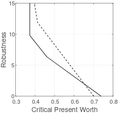
Figure 1: Robustness curve for loan portfolioP1.
Figure 2: Robustness curves for loan portfoliosP1(solid) andP2(dash).
A robustness curve
Fig. 1 shows a robustness curve for portfolioP1. The horizontal axis is the critical
present worth: the lowest value of expectedPW that would be acceptable to the
12One could argue that default probabilities all equal to unity is the worst possible case. That is true
bank. (ThePW has the same units as the client repayments, fkn.) The vertical
axis is the robustness: the greatest fractional error in the estimated probabilities of default that do not jeopardize the corresponding criticalPW. For instance, at a criticalPW of 0.6, the estimated default probabilities can err by a factor of 3 without jeopardizing thePW requirement.
Three concepts can be illustrated with this figure: trade off, cost of robustness, and zeroing. The negative slope demonstrates that the robustness decreases as the requiredPW increases. This expresses atrade off: as the requirement becomes more demanding (as criticalPW increases) the robustness becomes lower. More demanding requirements are more vulnerable to Knightian uncertainty than lax requirements. This is a generic property of info-gap robustness functions, and is sometimes called “the pessimist’s theorem”.
The curve in Fig. 1 expresses this trade off quantitatively, and the slope can be thought of as a cost of robustness. A very steep negative slope implies that the robustness increases dramatically if the requirement, criticalPW, is slightly reduced, implying a low cost of robustness. A gradual negative slope implies the opposite and entails large cost of robustness. From Fig. 1 we see that the cost of robustness is relatively high when the criticalPW is large (lower right). The cost of robustness actually becomes zero at the upper right when the slope is infinite. The robustness rises to infinity at low values of criticalPW in Fig. 1. Specifically, the robustness is infinite if the required present worth is less than the least possible value (this least possible value occurs when all risk-types default at midterm).
Which portfolio for the bank’s performance requirement? A preference re-versal
Figure 2 shows robustness curves for portfoliosP1 (solid) andP2 (dash). In P1the preponderance of clients are low-risk, while inP2the preponderance are
high-risk. The estimated default probabilities are the same for both portfolios, but less effort was invested in verifying the estimates forP1than forP2, which might
be justified by noting that the preponderance of clients inP1are low-risk in any
case. The repayment plan for low-risk clients are constant in time and the same in both portfolios. The repayment plans for high-risk clients decrease in time by moving more of the debt to early payments. Furthermore, inP2the repayments
are greater than inP1.
Fig. 2 shows that robustness vanishes at a greater value of criticalPW forP1
than forP2, as seen from the horizontal intercepts of the robustness curves. From
the zeroing property, this means thatP1’s estimatedPW is greater thanP2’s. If
these estimates were reliable (which they are not due to the Knightian uncertainty) then we would be justified in preferringP1overP2. Knightian uncertainty and
the zeroing property motivate the first methodological conclusion: do not prioritize portfolios according to their estimatedPWs.
The predictedPWs are not a reliable basis for portfolio selection because those predictions have zero robustness. Hence, we “migrate” up the robustness curve, trading criticalPW for robustness. At the lower right end of the curves we see that the cost of robustness is greater forP1than forP2(P2has steeper negative
slope). The differences in slopes and intercepts result in crossing of the robustness curves. This creates the possibility for areversal of preferencebetween the two portfolios. For instance, suppose the bank requires aPW no less than 0.7. From the solid curve we see that the robustness ofP1is 1.0 which exceeds the robustness
ofP2which is 0 at thisPW requirement. The robust-satisficing decision maker
would preferP1. However, if the bank can accept aPW of 0.6, thenP2is more
robust against Knightian uncertainty thanP1. The robust-satisficing prioritization
would now preferP2over P1. The robust-satisficing method implies that the
Note that the choice between P1 andP2 does not depend on specifying a
numerical value forPWc.P1is preferred for anyPWcexceeding the value at which
the robustness curves cross one another (about 0.65).P2is preferred for any other
value ofPWc.
It is important to understand why this preference reversal occurs. PortfolioP1
has relatively more low-risk clients than portfolioP2. Consequently, given the
parameterization assumed,P1would generate higher expected present worth if
there were no Knightian uncertainty and would be the portfolio to choose. However, it is also the portfolio that is less precisely measured. As discussed above, more effort has gone into estimating default probabilities for portfolioP2as expressed
by the lowersk jvalues in the info-gap model of Eq.(9). In other words, whileP2
would be worse thanP1if there were no Knightian uncertainty, the assessment
ofP2 is less uncertain. ThusP2 has lower estimated expected present worth
(intercept further left), butP2also has lower cost of robustness (steeper slope).
In short, there is a dilemma in the choice betweenP1andP2. The dilemma is
manifested in the crossing of the robustness curves. This crossing has the effect that, for moderate ambitions (anything below=0.65), portfolioP2satisfies these
ambitions for a greater range of default probabilities. The choice between the portfolios (and the resolution of the dilemma) depends on the decision maker’s choice of the critical present worth. Any value less than 0.65 is more robustly achieved withP2and this portfolio would be chosen, while any value greater than
0.65 would lead to choosingP1.
4 Robust satisficing vs min-max
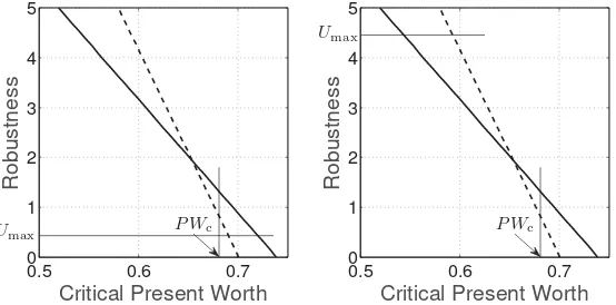
0.5 0.6 0.7
axis). LetUmaxdenote the min-max assessment of the maximum uncertainty, and
letPWc denote the robust-satisficing lowest acceptablePW.
Figs. 3 and 4 shows robustness curves for portfoliosP1(solid) andP2(dash),
from the lower-right portion of Fig. 2. A robust-satisficing decision maker’s least acceptable present worth,PWc, is labeled on the horizontal axis. The thin vertical
line on Fig. 3 shows that this analyst would preferP1(solid) overP2because P1is more robust against Knightian uncertainty for this requirement. A min-max
decision maker’s maximum possible uncertainty,Umax, is labeled on the vertical
axis. The thin horizontal line shows that this analyst would also preferP1(solid)
overP2because the worst outcome atUmaxis better withP1. The min-maxer and
the robust-satisficer agree on the prioritization of the portfolios, but for different reasons because their initial judgments differ. The min-maxer tries to ameliorate the maximal uncertainty; the robust-satisficer tries to achieve no less than an acceptable outcome.
Fig. 4 shows the same robustness curves but with a different judgment by the min-max analyst, who now identifies greater maximum possible uncertainty. The min-maxer now prefersP2(dash) because, at this largerUmax, the worst outcome
uncertainty could be as great asUmax. However, portfolioP2is less robust than P1for the specified critical outcomePWc, so the robust-satisficer still prefersP1
(solid). Now min-max and robust-satisficing prioritize the portfolios differently. The central ideas illustrated in this example are zeroing, trade off, preference reversal, and the situations in which min-max and robust-satisficing agree or disagree.Zeroingstates that predicted outcomes (estimated expectedPW in our example) have no robustness against Knightian uncertainty and therefore should not be used to prioritize the options. Trade off means that robustness increases as the performance requirement becomes less demanding. Robustness can be “purchased” by reducing the requirement, and the slope of the robustness curve quantifies the cost of robustness. The potential forpreference reversalbetween options arises when their robustness curves cross each other. The robust-satisficing analyst’s preference between the options depends on the outcome requirement. Finally, min-max and robust-satisficing both attempt to manage non-probabilistic Knightian uncertainty, but they are based on different initial judgments by the analyst, and they may either agree or disagree on prioritization of the options.
5 Trade-off revisited: Proxies for robustness in qualitative analysis
We now extend the discussion, in Section 3, of the trade-off between robustness and performance in a qualitative context. We discuss proxies for the concept of robustness that can support qualitative analysis, deliberation and debate, leading to selection of policy. Qualitative and quantitative analyses are not mutually exclusive. We first describe five conceptual proxies for robustness, and then briefly consider an example.
5.1 Five conceptual proxies for robustness
Thefive proxies for robustnessare resilience, redundancy, flexibility, adaptiveness and comprehensiveness. A policy has high robustness if it is strong in some or all of these attributes; it has low robustness if it is weak in all of them.
Resilienceof a policy is the attribute of rapid recovery of critical functions. Adverse surprise is likely when facing severe uncertainty. A policy is robust against uncertainty if it has the ability to rapidly recover from adverse surprise and achieve critical outcomes.
Redundancyof a policy is the attribute of providing multiple alternative solu-tions. Robustness to surprise can be achieved by having alternative policy responses available.
Flexibility(sometimes called agility) of a policy is the ability for rapid modi-fication of tools and methods. Flexibility or agility, as opposed to stodginess, is often useful in recovering from surprise. A policy is robust if its manifestation or implementation can be modified in real time, on the fly.
Adaptivenessof a policy is the ability to adjust goals and methods in the mid- to long-term. A policy is robust if it can be adjusted as information and understanding change. Managing Knightian uncertainty is rarely a once-through procedure. We often have to re-evaluate and revise assessments and decisions. The emphasis is on the longer time range, as distinct from on-the-spot flexibility.
Comprehensivenessof a policy is its interdisciplinary system-wide coherence. A policy is robust if it integrates considerations from technology, organizational structure and capabilities, cultural attitudes and beliefs, historical context, economic mechanisms and forces, and sometimes other factors. A robust policy will address the multi-faceted nature of the economic problem.
5.2 Policy examples
Consider the design offinancial architecture. We want banks to intermediate, take risks, invest, and contribute to growth. When economic circumstances are favourable, banks make profits and it is easy for them to perform their tasks. Moreover, when we thoroughly understand how the economy operates, it is possible to design regulation that will allow banks to perform their tasks optimally.
Good regulation, that is robust to uncertainty, will increase bankresilience:the abil-ity of banks to continue critical functions even after adverse surprise. For instance, a higher capital adequacy ratio gives banks greater resilience against unexpectedly large loss. A regulatory policy has beneficialredundancyif different aspects of the policy can at least partially substitute for one another as circumstances change. For example, banks’ lack of market access can be substituted by Central Bank liquidity provision as was made possible by Target 2 in the euro area. Beneficial
flexibilitycan be achieved by enabling short-term suspension of service, or central bank intervention, or other temporary measures. A policy has mid- to long-term
adaptivenessif it can be modified in response to longer-range changes. For in-stance, capital adequacy ratios need to be stable and known to market participants, but they may be adjusted from time to time to reflect assessments of increasing or decreasing systemic stability. Finally, thecomprehensiveness of a policy is expressed in its responsiveness to broad economic and social factors, and not only to local or institution-specific considerations.
We can now understand the trade-off between robustness (and its proxies) and the quality of the outcome achieved by banks. Several examples will make the point. Higher capital adequacy ratios will have higher resilience against adverse surprises, but lower profitability for banks and will result in less financial intermediation offered. Redundant controls, that ‘click in’ to replace one another as needed, provide greater protection against adversity, but constrain the ability of banks to be pro-active in their markets. Flexibility of the regulator (or of the regulation policy) enhances overall stability by enabling effective response to destabilizing bank initiatives that are motivated by adversity. However, flexibility of the regulator will tend to reduce bank profit and versatility and to impede planning by market participants.
in situations in which quantitative models are lacking. This is not to say that quantitative models are unneeded. Rather, the intuition behind the mathematics of quantitative analysis can be employed even when the math is absent.
This trade-off is also very prominent inmonetary policydiscussions. Mone-tary policy architecture in the past 20–30 years has relied on defining price stability and then announcing a target that best captures it. But the recent protracted pe-riod of low prices, as well as interest rates being at the zero lower bound, have challenged the merits of aiming at price stability altogether. The argument is that in-creasing the inflation target and therefore moving away from price stability, delivers a better buffer (greater resilience) from the very distortionary effects of disinflation and ultimately deflation. A trade-off therefore emerges between achieving price stability versus greater flexibility to deal with very distortionary negative shocks. At the same time, a higher inflation objective provides a greater choice of policies (greater redundancy) and indeed adaptability to unfavourable circumstances.
The method of info-gap robustness analysis captures this trade-off and allows policy makers to rank alternative policies. The absolute position of available policies in the robustness-vs-performance space, as well as the slope (i.e. the robustness gains when giving up performance by one unit) are powerful tools in the hands of policy makers to inform decision making.
6 Conclusion
min-max method then ameliorates this worst case, and does not require specification of an outcome requirement. Info-gap, in turn, does not presume knowledge of a worst case. We have also illustrated how conceptual proxies for the idea of robustness can be used in qualitative policy analysis.
The info-gap robust satisficing methodology quantifies an irrevocable trade-off between confidence (expressed as robustness to uncertainty) and performance (embodying the decision maker’s outcome requirement). This trade-off can be interpreted as a cost of robustness: robustness can be enhanced in exchange for reducing the performance requirement. The robustness curve characterizes any proposed policy as a monotonic plot of robustness versus performance requirement, where the slope reflects the cost of robustness and the horizontal intercept reflects the putative error-free outcome.
If the robustness curves of two alternative policies do not cross one another, then one policy is more robust than the other for all feasible outcomes. That robust-dominant policy is preferred, without the need to specify an outcome requirement. In this case, the putative optimum policy (whose estimated outcome is better) is also the robust-preferred policy.
If the robustness curves of two alternative policies cross one another, as seen in Fig. 2, then the robustness analysis can lead to a reversal of policy preference from the putative optimum. The policy that is more robust (and hence preferred) at high performance requirement, will be less robust (and hence not preferred) at lower requirement. Info-gap robust-satisficing leads to policy selection that will achieve the performance requirement over the greatest range of Knightian uncertainty.
References
Ben-Haim, Yakov (1999). Set-models of Information-gap Uncertainty: Axioms and an Inference Scheme,Journal of the Franklin Institute,336: 1093–1117. http://www.sciencedirect.com/science/article/pii/S0016003299000241
Ben-Haim, Yakov (2006).Info-Gap Decision Theory: Decisions Under Severe Uncertainty,2nd Edition, London: Academic Press.
Ben-Haim, Yakov (2010). Info-Gap Economics: An Operational Introduction,
London: Palgrave.
Ben-Haim, Yakov, Clifford C. Dacso, Jonathon Carrasco and Nithin Rajan (2009), Heterogeneous Uncertainties in Cholesterol Management,International Journal of Approximate Reasoning,50: 1046–1065.
http://www.sciencedirect.com/science/article/pii/S0888613X09000784
Ben-Haim Yakov and M. Demertzis (2008). Confidence in Monetary Policy, De Nederlandsche Bank Working Paper, No. 192, December.
https://ideas.repec.org/p/dnb/dnbwpp/192.html
Ben-Haim, Yakov, Craig D. Osteen and L. Joe Moffitt (2013), Policy Dilemma of Innovation: An Info-Gap Approach,Ecological Economics,85: 130–138. http://www.sciencedirect.com/science/article/pii/S0921800912003278
Blinder, Alan S. (1998).Central Banking in Theory and Practice,Lionel Robbins Lecture, Cambridge: MIT Press.
Brainard, W. (1967). Uncertainty and the Effectiveness of Policy,American Eco-nomic Review,57: 411–425.http://www.jstor.org/stable/1821642
Carmel Y. and Yakov Ben-Haim (2005). Info-gap robust-satisficing model of foraging behavior: Do foragers optimize or satisfice?, American Naturalist,
Chisholm, R.A. and B.A Wintle (2012). Choosing Ecosystem Service Invest-ments That Are Robust to Uncertainty across Multiple Parameters,Ecological Applications,22(2): 697–704. http://onlinelibrary.wiley.com/doi/10.1890/11-0092.1/full
Hansen, L. P., T. J. Sargent, G. A. Turmuhambetova, and N. Williams (2006). Robust Control and Model Misspecification,Journal of Economic Theory,128: 45–90.http://www.sciencedirect.com/science/article/pii/S0022053105001973
Hansen, L.P. and T.J. Sargent (2008).Robustness,Princeton: Princeton University Press.
Hildebrandt, Patrick and Thomas Knoke (2011). Investment Decisions under Un-certainty: A Methodological Review on Forest Science Studies,Forest Policy and Economics,13 (1): pp.1–15.
http://www.sciencedirect.com/science/article/pii/S1389934110001267
Kazemi, M., B. Mohammadi-Ivatloo, and M. Ehsan (2014). Risk-based Bid-ding of Large Electric Utilities Using Information Gap Decision Theory Con-sidering Demand Response, Electric Power Systems Research, 114: 86–92. http://www.sciencedirect.com/science/article/pii/S0378779614001564
Knight, F. H. (1921)Risk, Uncertainty, and Profit.Boston, MA: Hart, Schaffner & Marx; Houghton Mifflin Company
Nojavan, Sayyad, Hadi Ghesmati and Kazem Zare (2016). Robust Opti-mal Offering Strategy of Large Consumer Using IGDT Considering De-mand Response Programs, Electric Power Systems Research, 130: 46–58. http://www.sciencedirect.com/science/article/pii/S0378779615002540
Simon, H.A. (1955). A Behavioral Model of Rational Choice,Quarterly Journal of Economics,69: 99-118.http://www.jstor.org/stable/1884852
Simon H. A. (1957).Models of Man,New York: John Wiley and Son.
Sims, C.A. (2001). Pitfalls of a Minimax Approach to Model Uncertainty,American Economic Review,91 (2): 51–54.
https://www.aeaweb.org/articles.php?doi=10.1257/aer.91.2.51print=true
Stranlund, John K. and Yakov Ben-Haim (2008). Price-based vs. Quantity-based Environmental Regulation under Knightian Uncertainty: An Info-gap Robust Satisficing Perspective,Journal of Environmental Management,87: 443–449. http://www.sciencedirect.com/science/article/pii/S0301479707000448
Williams, N. (2007). Robust Control: An Entry for the New Palgrave, 2nd Edition.
Yokomizo, Hiroyuki, Hugh P. Possingham, Philip E. Hulme, Anthony C. Grice and Yvonne M. Buckley (2012), Cost-benefit Analysis for Intentional Plant Introductions under Uncertainty, Biological Invasions, 14: 839–849. http://link.springer.com/article/10.1007/s10530-011-0120-x
A A Special Case: One Default Time
We consider a special case for simplicity,Nd=2, meaning that if default occurs
then it happens at timet1. We derive an explicit analytical expression for the inverse
of the robustness function, ˆh, thought of as a function of the critical present worth,
PWc, at fixed loan portfolio(w,f). The analytical expression for the general case
is accessible but more complicated and is unneeded to achieve the goals of this example.
Define a truncation function:x+=xifx≤1 andx+=1 otherwise.
Letm(h)denote the inner minimum in the definition of the robustness function, Eq.(11).
A plot ofm(h)vshis identical to a plot ofPWcvs ˆh(PWc). Thusm(h)is the
inverse function of ˆh(PWc). Given thatNd=2, the expectation of the present worth,
Eq.(8), becomes:
From Eq.(12) and the info-gap model of Eq.(9) we see that the inner minimum in Eq.(11) is obtained, at horizon of uncertaintyh, when the probability of default of each risk type,pk1, is as large as possible. Thus:
andm(h) decreases piecewise-linearly ashincreases. Hence, sincem(h) is the inverse of the robustness function, ˆh(PWc), we see that ˆh(PWc) decreases
piecewise-linearly asPWcincreases.
Let E0denote the expectation of the present worth when each probability of default
Finally, definehmaxas the value of horizon of uncertainty,h, beyond which all the
probability terms[p˜k1+sk1h]+in Eq.(13) equal unity:
Now we find, from Eqs.(13)–(15), that:
m(h) =
piece-wise linearly decreasing if 0≤h≤hmax
E0 ifhmax<h.
(18)
From this relation we see that the robustness function has the following form:
ˆ
Please note:
You are most sincerely encouraged to participate in the open assessment of this article. You can do so by posting comments.
Please go to:
http://dx.doi.org/10.5018/economics-ejournal.ja.2016-23
The Editor