Full Terms & Conditions of access and use can be found at
http://www.tandfonline.com/action/journalInformation?journalCode=ubes20
Download by: [Universitas Maritim Raja Ali Haji] Date: 12 January 2016, At: 23:56
Journal of Business & Economic Statistics
ISSN: 0735-0015 (Print) 1537-2707 (Online) Journal homepage: http://www.tandfonline.com/loi/ubes20
Confidence Intervals for Half-Life Deviations From
Purchasing Power Parity
Barbara Rossi
To cite this article: Barbara Rossi (2005) Confidence Intervals for Half-Life Deviations From Purchasing Power Parity, Journal of Business & Economic Statistics, 23:4, 432-442, DOI: 10.1198/073500105000000027
To link to this article: http://dx.doi.org/10.1198/073500105000000027
View supplementary material
Published online: 01 Jan 2012.
Submit your article to this journal
Article views: 97
View related articles
Confidence Intervals for Half-Life Deviations
From Purchasing Power Parity
Barbara ROSSI
Department of Economics, Duke University, Durham, NC 27708 (brossi@econ.duke.edu)
Existing point estimates of half-life deviations from purchasing power parity (PPP), around 3–5 years, suggest that the speed of convergence is extremely slow. This article assesses the degree of uncertainty around these point estimates by using local-to-unity asymptotic theory to construct confidence intervals that are robust to high persistence in small samples. The empirical evidence suggests that the lower bound of the confidence interval is between four and eight quarters for most currencies, which is not inconsistent with traditional price-stickiness explanations. However, the upper bounds are infinity for all currencies, so we cannot provide conclusive evidence in favor of PPP either.
KEY WORDS: Half-life; Persistence; Purchasing power parity; Roots close to unity.
1. INTRODUCTION
What determines nominal exchange rates in the long run? According to Purchasing Power Parity (PPP), because the (bilateral) nominal exchange rate (Et) is the relative price of
two currencies (the bilateral nominal exchange rate is defined here as the price of the foreign country’s currency in terms of the home country’s currency), in equilibrium it should reflect their relative purchasing powers. So if Pt is the price level in
the home country andP∗t is the price level in the foreign coun-try, then PPP requires
Et=
Pt
P∗t . (1)
Thus the logarithm of the real exchange rate, defined as yt=ln(EtP
∗ t
Pt ), should be constant if PPP holds at every point in time. A weaker version of the PPP, which is followed in this article and in most of the literature, requires only that (1) holds in the long run.
The empirical evidence on PPP is mixed. Although casual evidence suggests that the two series,Et andPt/P∗t, tend to
re-vert toward each other over time, there are protracted periods in which the nominal exchange rate deviates from its PPP level. How persistent are these deviations? A measure of persistence is the half-life of PPP deviations. To motivate this measure, sup-pose that the deviations of the logarithm of the real exchange rateytfrom its long-run valuey0, which is constant under PPP,
follow an autoregressive process of order 1,
yt−y0=ρ(yt−1−y0)+ǫt, (2)
where ǫt is a white noise. Then, at horizon h, the
percent-age deviation from equilibrium is ρh. The half-life deviation from PPP is defined as the smallest value of h such that
E(yt+h−y0|yt−s−y0,s≤0)≤ 12(yt−y0), whereE is the
ex-pectation operator, that is,
ρh=1
2 ⇒ h=
ln(1/2)
ln(ρ) . (3)
Using data under floating exchange rate regimes, estimates of hrange between 2 and 5 years for most countries, with an av-erage of 3.7 years (see table 7.2 in Mark 2001). [Note that al-though these point estimates are introduced here to motivate the article, they no longer represent the current status of our knowl-edge; for example, Murray and Papell (2002) noted that after
accounting for serial correlation and small-sample bias, these point estimates become very difficult to believe.]
The existing point estimates of half-life deviations from PPP are difficult to reconcile with conventional explanations for the failure of short-run PPP based on price stickiness. Accord-ing to Rogoff (1996, p. 654), deviations from PPP can be at-tributed to transitory disturbances, like financial and monetary shocks, that buffet the nominal exchange rate and translate into real exchange rate variability because of nominal price stick-iness. Thus, whereas conventional explanations for the failure of PPP based on nominal prices stickiness are compatible with the enormous short-term volatility of real exchange rates, they also imply that deviations should be short-lived, because they can occur only during a time frame in which nominal wages and prices are sticky (i.e., 1–2 years). The existing point esti-mates imply instead that deviations are much more persistent than that. Rogoff (1996, p. 647) called this empirical inconsis-tency the “PPP puzzle.”
This article makes two contributions. First, it introduces a measure of the half-life for a general AR(p)process that al-lows better asymptotic approximations in the presence of a root close to unity. Although the methods for deriving the half-life are quite standard, there is no such result in the literature. Abuaf and Jorion (1990) discussed half-lives in the context of an AR(1) process only. Mark (2001) discussed measures of half-lives for general AR(p) processes, but for stationary processes only. Andrews (1993) proposed a measure of half-life for an AR(1)process that is robust to the presence of high persistence. Andrews and Chen (1994) generalized the method to obtain an approximate median-unbiased estimate of AR(p)
coefficients in the presence of high persistence. They showed how to construct an approximately median-unbiased estimator of the impulse-response function (IRF), but did not provide an analytic measure of the half-life for AR(p)processes.
Second, the article uses this measure to provide a simple method for constructing confidence intervals for the half-life. The issue is complicated by both the high persistence in real ex-change rates and the small samples usually available. For these reasons, this article considers an alternative asymptotic theory
© 2005 American Statistical Association Journal of Business & Economic Statistics October 2005, Vol. 23, No. 4 DOI 10.1198/073500105000000027 432
based on local-to-unity asymptotics and a half-life that grows to infinity at the rate of the sample size, as was done by Stock (1996) and Phillips (1998). How good this approximation is rel-ative to the conventional (normal sampling) asymptotic theory is explored in a Monte Carlo experiment.
This is not the first article on inference about half-life devi-ations from PPP. Authors who have recently addressed this is-sue include Cheung and Lai (2000), Murray and Papell (2002), Lopez, Murray, and Papell (2003), Gospodinov (2002), and Kilian and Zha (2002). All of these authors calculated confi-dence intervals by estimating impulse responses with various methods: Cheung and Lai (2000) relied on stationary, normal sampling distributions; Murray and Papell relied on work of Andrews and Chen (1994); Gospodinov (2002) relied on work of Hansen (1999); and Kilian and Zha (2002) used Bayesian methods. However, estimating the whole IRF may quickly be-come computationally intensive.
It is also important to note that there are different meth-ods for evaluating the persistence of a univariate AR process. One could rely on the cumulative IRF (which is directly related to the sum of the AR coefficients), as was done by Andrews and Chen (1994), or alternatively, one could focus on measur-ing the half-life, as in the present article. In the context of the PPP debate, it is appropriate to focus on the half-life, because that is one of the most important statistical measures used in the literature (see, e.g., the influential survey in Rogoff 1996). However, methods analogous to those used in this article could be adapted to the analysis of cumulative IRFs. It is important to note, however, that even if our method relies on a local-to-unity approximation for the largest root, it does not disregard short-run dynamics. In fact, our method approximates thewhole IRF to approximate the half-life. The short-run dynamics of the process is thus taken into account, although its sampling vari-ability is not, being of smaller order by the nature of the ap-proximation.
Overall, the results of this article are not inconsistent with tra-ditional explanations for the short-run failure of PPP, although they do not rule out infinite half-lives either. The existing point estimates, although too high to be reconciled with the PPP, also have huge variability. As a result, confidence intervals with 95% coverage for most currencies include four to eight quarters as their lower bound, a time interval in which deviations from PPP are compatible with nominal price and wage stickiness. How-ever, because we cannot rule out the possibility of an infinite half-life, we interpret the evidence as being simply not infor-mative enough.
The article is organized as follows. The next section in-troduces the data-generating process (DGP) considered and derives the measure of half-life used. Section 3 describes the methods used to construct the confidence intervals for h. Section 4 discusses a small Monte Carlo experiment that com-pares the coverage of the various confidence intervals discussed in Section 3. Section 5 discusses the empirical results, and Sec-tion 6 concludes.
2. MEASURING THE HALF–LIFE
Let the DGP for the log of the real exchange rate,yt, be
yt=dt+ut, t=1,2, . . . ,T, (4)
ut=ρut−1+vt,
wheredt=µ0is a deterministic component,vtis a mean-zero,
stationary, and ergodic process with finite autocovariances
γ (k)=Evtvt−k;ω2=+∞k=−∞γ (k)is finite and non-zero; and vt =b(L)−1ǫt, where ǫt is a martingale difference sequence
with finite fourth moments and constant varianceσǫ2andb(L)is finite order and hasp<∞(stable) roots. We do not allow the presence of a deterministic time trend in the theoretical DGP or in the empirical estimation. The reason for this is that if a deterministic time trend is present, then PPP in levels will not hold. (Note that if a deterministic trend is present, so that dt=µ0+µ1t, then the calculations that follow continue to
hold, provided that we define a time-varying long-run equilib-rium, that is, such that the long-run equilibrium at time τ is defined as yτ =µ0+µ1τ. This is the equilibrium path that
would have prevailed in the absence of the shock. The empiri-cal results for detrended real exchange rates are similar to those reported in this article and are available on request.)
To provide better asymptotic approximations to the statistics of interest in small samples when variables are highly persis-tent, we use local-to-unity asymptotic theory (see Stock 1991, among others),
ρ=ec/T≃1+c
T, (5)
where c is a constant (negative, if the process is highly per-sistent but mean-reverting) andT is the sample size. To provide better small-sample approximations in situations where the true half-life,h, can be “big” relative to the sample size, we derive the asymptotic distributions by lettinghincrease as the sample size T increases in such a way that their ratio remains a fixed numberδ, that is,
h
TT→→∞δ. (6)
We refer toδas the “half-life as a fraction of the sample size.” The persistence of the process in small samples, measured byc, is relevant for our purposes, because we are trying to esti-mate at which horizon the deviations from PPP are back to one-half after a shock. (We provide detailed empirical evidence on the degree of persistence in the bilateral exchange rates consid-ered in this article in the empirical section.) As we show later, the speed at which the effect of a shock dies away depends on a function of the largest root of the process,ρh, and, under as-sumption (6),
ρh →
T→∞e
cδ. (7) To derive an expression for the half-life in this general AR(p)
process, we need to derive an expression for the effect of the shockǫtonytafterhperiods. We derive it in terms of the
eigen-values of the process. [We follow Hamilton 1994 in referring to the inverse of the roots of the polynomialb(L)(1−ρL)as the eigenvalues (or the roots) of the DGP.] We factorize (4) as
(1−λ1L)(1−λ2L)· · ·(1−λpL)(yt−dt)=ǫt, (8)
where, for convenience,λ1=ρ is the root close to unity and
λ2, λ3, . . . , λp are the (stable) roots, the inverse of the roots
of the polynomial b(L). We also define λ to be a (p ×1)
vector containing all of the eigenvalues of the DGP, λ =
[λ1, λ2, . . . , λp]′. We assume that the eigenvalues are distinct.
Suppose that we start at time (t−1)in the long-run equilib-riumµ0, and at timetthere is a shockǫt. No other shocks hit the
economy subsequently. The shockǫt measures the initial
devi-ation from equilibrium, which we denote byyt≡yt−µ0=ǫt.
It follows that the deviation from equilibrium after h periods will beyt+h=c′λhǫt, wherecis a(p×1)vector with generic
to thehpower (see Hamilton 1994, p. 12). Afterhperiods, the percentage deviation from equilibrium relative to the initial per-centage deviation from equilibrium is
(yt+h−µ0)
(yt−µ0)
=∂yt+h
∂ǫt
=c′λh. (10)
(Recall that in this article, yt is thelogarithmof the real
ex-change rate, so yt+h−µ0 measures a percentage deviation.)
We call∂yt+h/∂ǫt (which is the usual definition of an impulse
response) “the effect of a shockǫtafterhperiods.” By
combin-ing (9) and (10) and isolatcombin-ing the largest rootλ1(=ρ), we have Because all eigenvalues except the first one are in modu-lus <1, as h→ ∞,λih+p−1→0 ∀i =1 so the second com-ponent in (11) disappears. Also, because by assumption p is finite, by combining (6) and (7), as T → ∞, we have that
λ1h+p−1=ρh+p−1=(1+Tc)h+p−1→ecδ (becauseρp−1→1). Also, asymptotically, λ1−λi≃1−λi ∀i =1. Notice finally
that(1−λ2)(1−λ3)· · ·(1−λp)=b(1). Thus the effect of the
shock afterhperiods is
∂yt+h
Note that this approximation assumes that there is only one root close to unity. It is possible to extend (12) to processes inte-grated of order higher than 1. In that case the second component in (11) becomes asymptotically relevant as well. However, the empirical evidence (see Table 4 in Sec. 5) suggests that there is only one root close to unity in real exchange rates, so we specialize the result to this case. In the Monte Carlo section we provide some sensitivity results to processes with a high second-largest root.
The half-life is defined as the horizonhat which the effect of the shock is one-half. Hence, from (12), we obtain that the half-life as a fraction of the sample size is
δ∗≡max so the half-life will be infinite with our long-horizon approxi-mation. In contrast, whenc<0, ln(1/2cb(1)) might be negative
when mean reversion is considerably fast. If this is so, then we letδ∗=0. In this case our method, which relies on (6), may not provide a good approximation. It follows that the half-life is
h∗≡max tionship betweenδ∗andcin (13). The monotonicity arises be-cause in the long run it is the root close to unity that is relevant. The monotonicity is not ensured if the autoregressive process is not persistent. Note that the proposed method does not require that the adjustment process be monotonic; the true DGP may have nonmonotonic behavior driven by the short-run dynamics inb(L), but these effects are of smaller magnitude at long hori-zons and impact the half-life (13) only through their cumulative effect,b(1).
Let us compare our measure of the half-life with those that one would get by running the regression in the form of an AR(1), thus ignoring short-run dynamics (as in Abuaf and Jorion 1990; Frankel and Rose 1996; Lothian and Taylor 1996), or by running the regression in augmented Dickey– Fuller (ADF) form and calculating the half-life on the basis of the coefficient on the lagged level variable only (see Mark 2001, par. 2.4, and references therein). The measure of the half-life in the former approach, call ithAR(1), would ignore the correction factorb(1), Comparing (14) with (15), it is clear that they will differ unless the true DGP is an AR(1), in which caseb(1)=1. [Note that even if the true DGP is an AR(p), the estimated coefficient in the AR(1)regression will be a consistent estimate of the largest root, becauseT(ρ−ρ)=(1
In the second approach, the researcher relies on estimates from the ADF regression. Following Stock (1991), the DGP (4), can be rearranged to yield the ADF regression
yt=µ0+α(1)yt−1+ which corresponds to an approximate half-life as a fraction of the sample size equal to
δa≡max Expression (17) has also been proposed by Andrews (1993) for the simple AR(1) case. Althoughα(1) is estimated from the (correct) AR(p) process, the half-life is calculated as if
α(1)were equal to the largest autoregressive root (ρ) in (2). By comparing (13) with (18), it is clear that again they will dif-fer unless the true DGP is an AR(1). The intuition behind this
result is that (16) is not the Sims, Stock, and Watson (1990) canonical representation, and this will matter at long horizons (see the App. for additional technical explanations and clarifica-tions). We report the biases in the various measures in a Monte Carlo simulation in Section 4, where we show that the biases inha andhAR(1) can be substantial and thath∗ is essentially unbiased.
3. ECONOMETRIC METHODS
After discussing different measures of half-lives, we address the issue of how to construct confidence intervals with the cor-rect coverage. First, it is well known thatb(1)can be consis-tently estimated by using the estimates from the ADF regression (see Stock 1991), so the correction factor can be consistently estimated by
b(1)= 1−
k
j=1 αj∗−1
. (19) Second, there are various methods for constructing confidence intervals for the root close to unity,ρ. In the remainder of this section, we discuss these and show how to construct confidence intervals for the half-life. The discussion that follows focuses on two-sided confidence intervals; the construction of one-sided confidence intervals follows in a straightforward way.
3.1 Confidence Intervals Based on Normal Sampling Distributions
Starting from (3) and a usual ADF regression (16), where ytis the real exchange rate, some empirical works estimate the
half-life to be
ha=
ln(.5)
ln(α(1)), (20)
where “hats” above a parameter denote its estimated value. Hence, using a delta method approximation, a conventional two-sided 95% confidence interval forha,(hal,hau), is
ha±1.96σα(1)
ln(.5)
α(1)
ln(α(1))−2
, (21) whereσα(1)is an estimate of the standard deviation ofα(1). 3.2 Confidence Intervals for Persistent Time Series
Based on Stock’s (1991) Method
Stock (1991) proposed a method for constructing confidence intervals based on median-unbiased estimates of the largest au-toregressive root of the process (4). Note that a given sam-ple size T and a given c identify the length of the half-life deviation, h, and that the true half-life as a fraction of the sample size, δ, is a monotone-decreasing function of c. It is then possible to construct a confidence interval for the half-life using the Stock (1991) method to construct a two-sided confidence interval forc,(cl,cu), and then, by monotonicity,
obtain a confidence interval for the half-life as a fraction of the sample size,(δl,δu), by applying (13) and (18). These can be
directly transformed to confidence intervals for the half-life,
(h∗l,h∗u) and (hal,hau), by multiplying by the sample size T. Similarly, the median-unbiased estimate of the half-life is ob-tained by using the median-unbiased estimate ofc, then apply-ing (13) and (18), and finally multiplyapply-ing the result byT.
3.3 Confidence Intervals Based on Elliott and Stock’s (2001) Method
In empirical applications, Stock’s method may deliver wide confidence intervals. The reason for this is that it is based on inverting the ADF test statistic, which has poor power proper-ties (see Elliott, Rothemberg, and Stock 1996). Another draw-back of Stock’s approach is that it allows the construction of a confidence interval by inverting a statistic for testing whether c=0; in general, it might be interesting to test other null hy-potheses. Elliott and Stock (2001) discussed how to build con-fidence intervals based on the point-optimal test proposed by Elliott et al. (1996) and for more general null hypotheses. This section builds on their results.
To construct the confidence interval, we follow Elliott and Stock (2001) and invert a sequence of test statistics, with each test statistic being the point-optimal one for testingH0:c=c0.
We chose the coverage of the confidence interval constructed in this way to be at least 95%. The lag length in the test statistic is chosen according to the Modified Akaike Information Crite-rion (MAIC) criteCrite-rion based on generalized least squares (GLS) detrended data, as suggested by Ng and Perron (2001).
3.4 Hansen’s Grid-Bootstrap Method
An alternative method for constructing confidence intervals is the bootstrap. However, as Hansen (1999) showed, the prob-lem with conventional bootstrap methods is that even in large samples, their coverage probability is quite poor if the true value of the highest autoregressive root is close to unity and that root is the parameter of interest.
A bootstrap method that is valid in the presence of highly per-sistent variables is Hansen’s (1999) grid-αbootstrap method. Because the half-life is a monotone transformation of the ADF parameters, by the transformation-respecting property of the percentile method, we can construct a confidence interval for the half-life by taking the monotone transformation of the cor-responding confidence interval forα(1). Furthermore, by the range-preserving property of the grid-αmethod, the constraint that the half-life cannot be negative directly translates into a constraint on α(1)[namelyα(1)≤1], so it will be automati-cally satisfied. Hansen (1999) also suggested a grid-tbootstrap method. However, the half-life is a nonlinear transformation of the parameterα(1). In practice, the grid-tmethod requires an estimate of the variance, which, if obtained by the delta-method approximation, makes the coverage quite poor. (Results of a Monte Carlo experiment are available on request.) Also, con-structing confidence intervals by minimizing their length gave similar empirical results.
As emphasized by Stock (1991), the first-order asymptotic theory described in Section 3.1 does not provide a suitable framework for the construction of confidence intervals, because it is discontinuous atρ=1. This motivates the construction of confidence intervals forh based on confidence intervals forc obtained by using the procedures described in Sections 3.2–3.4. The procedure of Section 3.2 is expected to provide better ap-proximations than the usual normal sampling theory whenρis close to 1. This is based on the conjecture that the inversion of the ADF test statistic to form confidence intervals will work bet-ter than normal sampling for small|c|. Thus the performance of
the proposed method will depend onρ(it will work better forρ
close to 1) and on the magnitude ofhrelative toT (the larger his relative toT, the better the procedure). In particular, the the-ory does not imply that the confidence intervals will have good coverage for ever-growing sample sizes for a fixed value of h. However, for some intermediate combinations of parameter val-ues and sample sizes, the proposed procedure may work well. Only Monte Carlo evidence will establish how good these ap-proximations are, and the next section provides such evidence. It is important to emphasize that both the absolute performance and the relative performance (relative to that of other available methods) are important.
4. A SMALL MONTE CARLO EXPERIMENT
To evaluate the performance of the methods used in this ar-ticle, we performed some small Monte Carlo experiments. The experiments are useful to address two questions: (1) How big does the true half-life have to be for the Th →δ asymptotics to be better than the usual asymptotics, and (2) how does serial correlation inb(L)affect the performance of different methods. In the first experiment, data are generated asyt=ρyt−1+ǫt,
ǫt∼N(0,1), andρ=(1+Tc), and we compare the coverage of
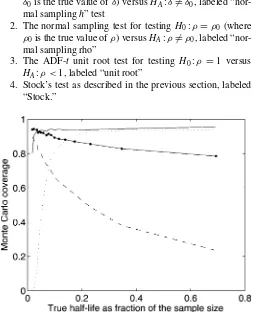
the confidence intervals for different values of the true half-life as a fraction of the sample size,δ. The number of Monte Carlo replications is 5,000, and the sample size is T=100. Results are reported in Figure 1.
The figure compares confidence intervals based on four tests: 1. The normal sampling test for testing H0:δ=δ0 (where
δ0is the true value ofδ) versusHA:δ =δ0, labeled
“nor-mal samplingh” test
2. The normal sampling test for testingH0:ρ=ρ0(where
ρ0is the true value ofρ) versusHA:ρ =ρ0, labeled
“nor-mal sampling rho”
3. The ADF-t unit root test for testing H0:ρ=1 versus
HA:ρ <1, labeled “unit root”
4. Stock’s test as described in the previous section, labeled “Stock.”
Figure 1. Comparison of Coverage of Various Confidence Intervals as a Function of the True Half-Life (nominal coverage=.95; nor-mal samplingρ; normal sampling h; unit root; Stock).
Table 1. Comparison of Coverage Rates
h c Normal Unit root Stock Elliott–Stock Hansen
2 −30 .718 .00 .91 .92 .96 6 −11.5 .710 .59 .93 .97 .92 20 −3.5 .468 .91 .94 .97 .96 +∞ −.01 .020 .95 .96 .96 .95
NOTE: The table reports, for each true half-life (and its corresponding measure of persistence in the data, “c”) is the coverage rate of the confidence intervals based on: approximate normal sampling distribution (“Normal”); unit root test (“Unit root”); Stock (1991) method (“Stock”); Elliott and Stock (2001) method (“Elliott–Stock”); Hansen (1999) grid-αbootstrap method (“Hansen”). Ideally, these coverage rates should be close to .95. In the case of multiple intersections between the estimated test statistic and the critical values, we convexified the confidence interval. In the case of Stock’s method, we simulated the critical values of the ADF test statistic outside the range considered by Stock (1991). The number of Monte Carlo simulations was 5,000 for all methods except Hansen, which is computationally intensive, so we chose 100 Monte Carlo replications only. HereT=100, and the lag length is assumed to be known.
As expected, the coverage of the normal sampling confidence intervals is fine when the half-life is small relative to the sam-ple size (δis smaller than .02, say); however, when the half-life is big, then the normal sampling test rejects too often and, as a consequence, coverage is lower than nominal. [Note that the same problems would arise if one were to construct the confi-dence intervals based on IRFs without taking into account the persistent nature of the process.] The problem with unit root tests, instead, is that they lack power. Finally, notice that con-fidence intervals based on Stock’s method have coverage close to nominal for most true half-lives (unless they are consider-ably short).
We also compared the performance of the various methods that are robust to high persistence in another small Monte Carlo experiment. We generated the data as before for four differ-ent true half-lives: 2, 6, 20, and infinity. (In practice, the infi-nite half-life is 6,900, corresponding to a value ofc= −.01.) Table 1 reports the results. Notice that the coverage of the confidence interval based on normal sampling asymptotic the-ory (labeled “Normal”) tends to 0 ash increases and is pretty poor relative to, say, that based on the method of Stock (1991) even for very small half-lives. Similar results hold for the grid-bootstrap and the method of Elliott and Stock (2001).
Finally, Table 2 compares confidence intervals based on dif-ferent methods in simple AR(p)processes (p=2,3,4,6) de-scribed by (8) for sample sizes usually available for quarterly real exchange rates (T =100). We compare confidence inter-vals based on the following methods: Stock applied to (14) (la-beled “Stock”) and Stock applied to (17) (labeled “ADF”). The table reports the actual confidence interval type I error, which ideally should be .10. Stock’s method performs well as long as the roots other thanρare not too close to unity [because oth-erwise the second component in (11) becomes asymptotically nonnegligible]. The performance of the ADF method wors-ens as the amounts of serial correlation increases. Some of the DGPs are calibrated on actual estimates: AR(2)withλ2= −.2
corresponds to Spain; AR(3)withλ2= −.27 andλ3=.13
cor-responds to Italy; AR(4)withλ2= −.68 andλ3=λ4=.2
cor-responds to Denmark (results are similar for Belgium); AR(6)
withλ2=λ3= −.6,λ4=λ5=.2, andλ6=.5 corresponds to
Sweden (results are similar for Finland and Japan); and AR(6)
withλ2=λ3= −.6,λ4=λ5=.34, and λ6=.3 corresponds
to Greece. Table 2 shows that for the latter case, usingharather
thanh∗ may lead to slightly higher confidence interval type I
error. Most countries with AR(2)processes have a very small
Table 2. Comparison of Actual Confidence Interval Type I Error
c λ2 λ3 λ4 λ5 λ6 h Stock ADF h∞
−5 −.2 10 .10 .12 .14
−8 −.2 6 .12 .15 .25
−11.5 −.2 5 .09 .11 .42
−5 −.27 .13 12 .10 .11 .12
−8 −.27 .13 8 .09 .10 .22
−11.5 −.27 .13 5 .11 .14 .36 −5 −.68 .2 .2 13 .09 .10 .12
−8 −.68 .2 .2 8 .09 .11 .20
−11.5 −.68 .2 .2 5 .15 .18 .31 −5 −.6 −.6 .2 .2 .5 10 .17 .17 .10 −5 −.6 −.6 .34 .34 .3 37 .15 .14 .09 −8 −.6 −.6 .2 .2 .5 2 .14 .13 .14 −8 −.6 −.6 .34 .34 .3 39 .12 .11 .14 −11.5 −.6 −.6 .2 .2 .5 25 .12 .12 .21 −11.5 −.6 −.6 .34 .34 .3 46 .12 .11 .20
NOTE: Monte Carlo simulations (5,000) replications are based on the AR(p) process (p=2, 3, 4, 5) described by (8). Here,T=100. The table reports the actual confidence inter-val type I error based on the Stock (1991) method forh∗(“Stock”) and forha(“ADF”). Ideally, these percentages should be close to .10. The table also reports the true half-life,h, and the em-pirical fraction of times in which the upper bound of the confidence interval based on the Stock (1991) method forh∗rejects an infinite half-life; that is, it rejects a unit root (labeled “h∞”). The lower bound was almost always below infinity. Whenλ=0∀i, coverage is close to nominal for all methods. The lag length is treated as known is all methods.
second root, usually smaller than .2 in absolute value, for which the two methods provide similar results. Thus, looking ahead to Section 5, for most currencies the serial correlation is so small that the two methods are expected to give similar results (except for Sweden, Spain, and Canada).
Evidence on the coverage properties of our method is not sufficient to conclude that the method is reliable, because we would also like the confidence intervals to exclude an infi-nite half-life with sufficient probability. Table 2 also reports evidence on the empirical proportion of times in which the con-fidence interval based on work of Stock (1991) does not in-clude an infinite half-life (labeled “h∞”). The table shows that
our method can potentially rule out an infinite half-life, and, for given values of the short-run serial correlation, these re-jections are more likely with increasingly stationary true DGP. For example, in the AR(2)case (Spain), rejection frequencies corresponding to values ofcaround the lower bound of the con-fidence interval (around−11.5) can be as high as .40. Finally, Table 3 shows that for a given value ofρ, rejection rates become closer to 1 as the sample size increases.
Finally, to investigate the biases in the various measures of the half-life, we simulated (8) in a simple AR(2)case, where
λ1=1+Tc andb(L)=(1−λ2L). The lag length is assumed
Table 3. Comparison of Actual Confidence Interval Type I Error (upper bound of the confidence interval) for Various Values of T
T=250 T=500
ρ λ2 h∞ ρ λ2 h∞
.95 −.2 .47 .95 −.2 .97 .92 −.2 .85 .92 −.2 .99 .885 −.2 .99 .885 −.2 1 ρ λ2,λ3 λ4,λ5 λ6 h∞ ρ λ2,λ3 λ4,λ5 λ6 h∞
.95 −.6 .2 .5 .34 .95 −.6 .2 .5 .87 .92 −.6 .2 .5 .61 .92 −.6 .2 .5 .99 .885 −.6 .2 .5 .83 .885 −.6 .2 .5 1
NOTE: Monte Carlo simulations (5,000 replications) are based on the AR(p) process (p=2, 3, 4, 5) described by (8). The notation in this table is the same as in Table 2. This ta-ble reports only a representative subset of the parameters examined in Tata-ble 2.
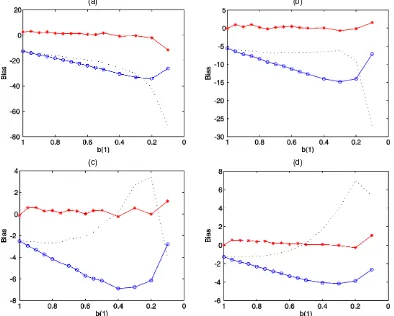
to be known, and the sample size is 100. Figure 2 compares the absolute values of the median biases of the various mea-sures of the half-life considered in Section 2,h∗namely,hAR(1), andha, as a function of b(1). The biases are measured in the
same units ofh. The figure shows thath∗is unbiased, whereas haandhAR(1) have substantial biases that depend both on the persistence of the series (“c”) and on the additional serial cor-relation (“b(1)”). In some cases where persistence is very high, the biases can be as high as 30 periods forhaand 70 forhAR(1) [Fig 2(a)]. Note thathaandhAR(1)are biased even ifb(1)=1; this is due to the downward bias in the estimate of the largest root that appears in (17) and (15). In unreported additional Monte Carlo simulations, we further compared the lengths of the confidence intervals obtained by using the various meth-ods. As one would expect, because the method of Elliott and Stock (2001) inverts a point-optimal test, it delivers the small-est confidence intervals, unless the process is not very persis-tent. The method of Hansen (1999) delivers confidence intervals of smaller length than those obtained by the method of Stock (1991), although the differences are minor.
5. EMPIRICAL RESULTS
The data used in this article are from Datastream (IMF Data-base). Data on the nominal exchange rate are end-of-period, and data on prices are seasonally unadjusted, to avoid tempo-ral aggregation issues (as discussed in Taylor 2001). The nom-inal exchange rate is expressed as national currency units in terms of 1 U.S. dollar (i.e., the price of dollars in terms of other national currency units). Data are quarterly from 1973:3 to 2002:2 for non-EMU countries and from 1973:3 to 1998:2 (for a total of 100 observations) for EMU countries. The price indices are consumer price indexes (CPIs), so they do not distin-guish between tradables and nontradables. The log of the real exchange rate is constructed as the log of the bilateral nom-inal exchange rate plus the log of the CPI in the U.S. minus the log of CPI in the reference country. The series used are “XXI64. . .F” (CPI) and “XXI. . .AE.” (bilateral nominal ex-change rate), where “XX” is the mnemonic used by the IMF to denote the country (e.g., “US” for the U.S.).
Table 4 reports confidence intervals based on standard as-ymptotic theory. The lag length of the ADF test statistic is chosen by the MAIC criterion based on ordinary least squares (OLS) demeaned data. Because the half-life cannot be nega-tive, we imposed a lower bound of 0 (which implies immediate adjustment). According to the table, point estimates ofh∗ are around 8–12 quarters (2–3 years) for most currencies. As dis-cussed previously, researchers used to reportha. From Table 4,
notice that, due to the absence of the correction factor, this procedure generally underestimates the true half-life. [To save space, confidence intervals forh∗are not reported. They gener-ally comprise higher values for the half-life. We chose to report confidence intervals based onhato make the results comparable
with those reported in the literature.]
Based on normal sampling asymptotic theory, the 95% nor-mal confidence intervals include 0–20 (or more) quarters for most currencies. However, the real exchange rate is a highly persistent series. In fact, Table 4 also reports the conventional ADF tests for the real exchange rate series. Because the 5%
(a) (b)
(c) (d)
Figure 2. Comparison of Median Biases of the Various Measures of the Half-Life as a Function of b(1). (a) c= −3; (b) c= −5; (c) c= −8; (d) c= −11.5 ( h∗; h
a; hAR(1)).
critical value is−2.89, we cannot reject the null hypothesis that there is a unit root in any of the currencies considered, and thus that the PPP does not hold. The table also reports the Dickey–
Table 4. Confidence Intervals Based on Standard Asymptotics and ADF Tests
α(1) ADF ADFGLS ha (hla,hua) h∗ γ Austria .936 −1.8 −1.79 10.4 (0; 22.1) 10.4 Australia .962 −1.4 −.37 18 (0; 43) 18 Belgium .932 −2.07 −2.1 10 (0; 20) 10.4 .1 Canada .99 −.588 −.39 66.6 (0; 290) 66.6 Denmark .92 −2.34 −2.39 8.55 (1; 16) 9 .1 Finland .91 −2.17 −2.1 8.15 (0; 15) 8.24 .3 France .932 −1.83 −1.72 9.92 (0; 20.9) 9.92 .1 Germany .936 −1.81 −1.67 10.6 (0; 22.4) 10.6 Greece .929 −1.97 −2.04 9.36 (0; 19) 9.9 Italy .921 −2.02 −2.03 8.45 (0; 17) 8.86 .2 Japan .93 −2.16 −1.2 10.8 (.6; 20.9) 11.4 .1 Netherl. .928 −1.89 −1.81 9.32 (0; 19.4) 9.32 .1 Norway .931 −1.99 −2 9.72 (0; 19.6) 9.72 Spain .947 −1.8 −1.64 12.8 (0; 27.1) 13.5 .2 Sweden .951 −1.71 −1.24 13.8 (0; 26.5) 14.6 .2 Switzerland .913 −2.33 −1.75 7.66 (.9; 14.4) 7.6 U.K. .913 −2.34 −1.65 7.61 (.75; 14.1) 7.61 .2
NOTE: For each bilateral real exchange rate, we report the estimated test statistic of the demeaned ADF regression (ADF), the estimated coefficient of the lagged regressor [α(1) as defined in (16)], and the DF–GLS test proposed by Elliott, Rothemberg, and Stock (1996) (ADFGLS). The lag lengths are selected by the MAIC criterion based on the OLS and on the GLS detrending methods proposed by Ng and Perron (2001).haandh∗are the estimates of the half-life from (17) and (14); (hl
a,hua) is based on (21). The 5% critical value of both theADF andADFGLStest statistics is−2.89.γis the absolute value of the estimated second-largest root (significantly less than 1 for all countries).
Fuller GLS–efficient test statistic of Elliott et al. (1996), which is more powerful for rejecting the null hypothesis of a unit root. However, even this test does not reject the hypothesis that the real exchange rate is not mean-reverting. But although one can-not reject that the half-life can be infinity, these results do can-not determine how low the lower bound for the estimated half-life can be. To answer this question, the remainder of the article fo-cuses on the construction of confidence intervals that are robust to highly persistent variables.
Table 5 shows the estimated confidence intervals for h∗ and ha based on Stock’s method. We report only the lower
bounds of the confidence intervals, because the upper bounds were infinity for all currencies. For a few currencies, also the median half-life is infinity. However, the uncertainty over the estimated half-life is so big that a half-life of six to eight quar-ters is compatible with the observed data for almost all cur-rencies as well. The most notable exception is the Canadian real exchange rate; however, the data clearly show that there is a time trend in that case. Other countries for which the lower bound of the half-life is quite high are Australia and Sweden. But for most countries, the lower bound is less than eight quar-ters anyway. Thus on the one hand, the upper bounds can be as high as infinity, invalidating PPP; on the other hand, the lower bounds are compatible with a time horizon in which prices may be sticky and thus horizons in which short-run deviations from PPP might be explained in light of monetary and financial shocks (a possible resolution of the “PPP puzzle”). The
Table 5. Confidence Intervals Based on Stock (1991)
lags (cl,cu) cl.05 ha.05 hmediana b(1) h∗.05 h∗median
Austria 1 (−12.5; 3.67) −10.93 6.34 29.96 1.00 6.34 29.96 Australia 1 (−8.87; 4.13) −7.53 10.67 +∞ 1.00 10.67 +∞ Belgium 4 (−15.5; 3.13) −13.8 7.91 21.42 .63 8.31 22.51 Canada 1 (−3.06; 4.74) −1.75 45.97 +∞ 1.00 45.97 +∞ Denmark 4 (−18.6; 2.67) −16.85 7.16 15.72 .66 7.56 16.62 Finland 6 (−16.6; 2.95) −14.93 8.9 21.9 .52 9.00 22.14 France 1 (−12.8; 3.62) −11.23 6.17 26.48 1.00 6.17 26.48 Germany 1 (−12.5; 3.66) −10.97 6.32 29.50 1.00 6.32 29.50 Greece 6 (−14.3; 3.36) −12.66 8.08 25.26 .67 8.55 26.73 Italy 3 (−14.9; 3.24) −13.21 6.14 17.76 .85 6.44 18.63 Japan 6 (−16.4; 2.98) −14.74 7.43 18.55 .73 7.89 19.69 Netherl. 1 (−13.4; 3.53) −11.82 5.86 21.47 1.00 5.86 21.47 Norway 1 (−14.6; 3.3) −12.93 6.22 18.66 1.00 6.22 18.66 Spain 2 (−12.4; 3.67) −10.88 8.00 38.66 .79 8.47 40.9 Sweden 6 (−11.5; 3.78) −10.04 11.9 91.85 .67 12.6 97.11 Switzerland 1 (−18.6; 2.68) −16.79 4.78 10.5 1.00 4.78 10.54 U.K. 1 (−18.7; 2.66) −16.9 4.75 10.42 1.00 4.75 10.42
NOTE: For each bilateral real exchange rate, we ran a demeanedADFregression. The median-unbiased two-sided and one-sided confidence intervals forc, denoted by (cl,cu) andcl.05, are obtained directly by inverting Stock’s table A1 (with a linear interpolation from its grid values). We report one-sided lower bounds for the median unbiased confidence intervals for the half-life (h) with coverage .95, denoted by subscript .05. Superscripts∗andadenote measures of the half-life obtained by multiplying (13) and (18) (based onc.05
l ), byT, whereTis the sample size. Upper bounds were+∞for all currencies, so they are not reported.
hmedianis the median unbiased estimate of the half-life (based on the median unbiased estimate ofc).
dence intervals are thus too wide to provide conclusive support in favor of the PPP.
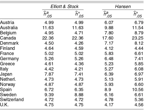
Table 6 reports the confidence intervals based on the meth-ods of Elliott and Stock (2001) and Hansen (1999). According to our estimates, the lower bounds for the half-life deviations from PPP are between four and seven quarters for most curren-cies, except for a few outliers (Canada and Australia). Overall, this additional evidence delivers confidence intervals of roughly the same magnitude as Stock’s method, thus confirming the pre-vious results.
It is important to note that it is not just low power of the tests that lets half-lives that accord with sticky price models into the confidence interval. In fact, in unreported Monte Carlo simulations, the methods of Stock and Elliott and Stock both have substantial rejection probabilities against false half-lives,
Table 6. Confidence Intervals Based on Elliott and Stock (2001) and Hansen (1999)
Elliott & Stock Hansen
ha.05 h∗
.05 h.05a h∗.05 Austria 4.99 4.99 6.07 6.79 Australia 11.63 11.63 9.88 11.54 Belgium 4.95 4.71 7.80 8.79 Canada 22.36 22.36 17.60 23.25 Denmark 4.50 4.26 7.17 8.12 Finland 4.64 4.59 4.12 4.44 France 5.02 5.02 5.83 6.61 Germany 5.26 5.26 6.48 7.41 Greece 4.61 4.36 5.23 5.85 Italy 4.42 4.21 5.27 6.08 Japan 7.87 7.41 6.39 6.97 Netherl. 4.73 4.73 5.13 5.91 Norway 4.87 4.87 5.93 6.60 Spain 6.72 6.35 8.9 10.56 Sweden 9.39 8.88 6.16 6.61 Switzerland 4.72 4.72 4.78 5.36 U.K. 4.75 4.75 4.17 4.56
NOTE: For each bilateral real exchange rate, we ran a demeanedADFregression, where the lag length is chosen according to MAIC. We report the one-sided confidence intervals for the half-life (h) with coverage .95, denoted by subscript .05. Superscripts∗andadenote measures of the half-life in equations (14) and (17). Upper bounds were infinity for all currencies, so they are not reported.
and in particular they have higher rejection probabilities against smaller half-lives than against higher half-lives. For example, when the true half-life is 7, the probability to reject a half-life of 4 is around 30% and becomes 60–70% against a half-life of 2. When the true half-life is 14, the probability to reject a half-life of 5 is around 30% and becomes 70–80% against a half-life of 2, and similar remarks hold for a true half-life equal to 35.
6. CONCLUSIONS
The objective of this article was to propose a better approx-imation to the half-life for highly persistent processes in the presence of small samples and to use it to build confidence in-tervals for half-life deviations from PPP. We first showed that normal sampling methods for constructing confidence intervals might be unreliable when variables are highly persistent and the sample size is small. Because the empirical evidence suggests that the real exchange rate is such a variable, we then consider methods that are robust to persistence. These methods (Stock, Elliott and Stock, and Hansen) imply confidence intervals that cover half-lives as low as five to eight quarters for most real ex-change rates considered in this article (although some countries are outliers).
Overall, the results of this article suggest that the real ex-change rate is a highly persistent variable and that the confi-dence intervals for the half-life are extremely wide. On the one hand, they are compatible with processes that can halve in four to eight quarters, and thus consistent with conventional price-stickiness explanations for the PPP puzzle. On the other hand, they do not rule out the possibility of an infinite half-life. The empirical results thus show that the data are not informative enough to support any alternative hypothesis regarding the half-life based on the tests used in this article. This is likely due to the limited power of the unit root tests and the short data that we use. This conclusion is similar to that of Murray and Papell (2002) and Kilian and Zha (2002). In the work of Kilian and
Zha (2002), for example, the Bayes factors, which provide use-ful results beyond what a confidence or posterior probability interval gives, similarly imply that the data are not informative enough. More powerful tests might be able to provide more em-pirical support for the PPP. For example, Elliott and Pesavento (2001) applied higher-power tests for mean reversion against close alternatives by exploiting information on other economic variables.
Some researchers have recently addressed the question of size distortions of tests in the presence of persistent real ex-change rates and their implications for the PPP debate (see Engel 2000; Caner and Kilian 2001). However, Caner and Kilian focused on size problems of tests of the null hypothesis of stationarity versus the alternative of a unit root. Engel (2000) discussed both tests on a unit root and tests on stationarity, but focused on simulations (calibrated on real data) to show the ex-istence of possible size distortions in the former and low power in the latter.
This article assumes a linear DGP. Recent research also points to nonlinearities as a possible explanation for the ap-parent high persistence and excess volatility of exchange rates (e.g., Taylor 2001, 2002; Shintani 2002). Furthermore, this ar-ticle does not address panel issues, nor does it consider longer datasets that merge floating and fixed exchange rate samples. We would expect panel tests and tests based on longer data se-ries to have more power to reject a unit root and hence confi-dence intervals obtained by inverting these tests to strengthen the empirical evidence in favor of PPP. However, this would require additional assumptions on the joint distribution and a careful investigation of cross-sectional dependence (O’Connell 1998). Finally, it might be worth investigating potential aggre-gation biases (as in Imbs, Mumtaz, Ravn, and Rey 2002) and the reasons why some countries’ half-lives are much higher than others’. However, all of these questions are left for future re-search.
ACKNOWLEDGMENTS
The idea of this article came out during discussions with Mark Watson, whom the author thanks for many valuable suggestions and continued support. The author also thanks Bo Honore, Tim Bollerslev, Graham Elliott, Charles Engel, Christian Murray, Marcelo Mello, Ulrich Muller, the associate editor, two referees, and seminar participants at the University of Virginia, University of North Carolina, Emory University, the 2002 Summer Meetings of the Econometric Society, the 2002 Midwest Econometric Group Conference, and the 2002 Triangle Econometrics Conference. Financial support provided by the IFS, Princeton University, is gratefully acknowledged. Any mistakes are the authors’.
APPENDIX A: COMPARISON OF EXACT AND APPROXIMATE HALF–LIVES WITH AN APPLICATION TO AN AR(2) PROCESS
We compare three candidate measures of the long-run effects of a unitary shock: (a) the AR(1) long-run effect, which de-pends only on the largest unit root of the process and not on short-run dynamics, equal toρh; (b) theapproximate long-run
effect, frequently used by applied researchers, equal toα(1)h; and (c) theexact long-run effect, proposed in this article, equal toρhφb, whereφb≡b(1)−1. To highlight the relationship
be-tween the approximate and the exact long-run effects, we re-arrange the ADF regression (16) as
yt=
An alternative approach is to follow Stock (1991) and Phillips (1998) in rewriting the ADF regression in terms of the canonical regressors. We call this theADF canonical re-gression. The canonical regression approach was introduced by Sims, Stock, and Watson (1990); it corresponds to a trans-formed DGP where all of the regressors (in the representation foryt) except one have mean 0 and are stationary,
yt=ρyt−1−
whereE11=ρ and the rest of the matrix Eis partitioned
ac-cordingly,Yt≡ [yt,yt,yt−1, . . . ,yt−k+1]′is a(k+1)×1
vector, andyt−j≡yt−j−ρyt−j−1. We also find it convenient
to define1kto be the first column of the(k×1)identity matrix andIkto be the identity matrix withkelements.
Suppose that we start at timet−1 in the long run equilib-riumyLRt−1, and at timetthere is a shockǫt. The initial deviation
from equilibrium is thus
yt=1′ket=ǫt. (A.7)
By using (A.5), the effect of the shock in the subsequent periods
Hence, afterhperiods, the percentage deviation from rium relative to the initial percentage deviation from equilib-rium is This measures the effect of a shock ǫt after h periods. The
usefulness of the foregoing VAR(1)representation is that be-cause ρ −1 =c/T, it follows that E21 ≃0k×1, so that E
(as partitioned) is asymptotically an upper-diagonal matrix. As a consequence, cally), which imply that(E22/E11)h also vanishes
asymptoti-cally. Hence the effect of the shock on the first component ofYt
afterhperiods,Eh[1,1,01×(k−1)]′, will be equal to
where in the last line we use the approximation thatE11=ρ=
1+Tc ≃1. Thus
whereφbis the correction factor,
φb≡1+E12(Ik−E22)−11k. (A.13)
It can be shown that this is the same correction factor derived in Section 2. This is the reason why we call it in the same way. (See Hamilton 1994, chaps. 1 and 2, for a discussion on the equivalence of the eigenvalue factorization and the VAR repre-sentation.) We do not prove this here, but only show that this is true in the AR(2)example that follows.
We could repeat the same reasoning for the matrix A. By
doing the same calculations, we find that for the ADF regres-sion (A.1), the long-run effect is
where the correction factor is
φα∗≡1+A12(Ik−A22)−11
k. (A.15)
To highlight the differences between the two results, we in-troduce a simple example. We consider an AR(2)process with-out deterministic components,
The canonical ADF representation is
yt=ρyt−1+γ (yt−1−ρyt−2)+ǫt. (A.19)
Finally, the ADF representation is
yt=α(1)yt−1−ρ2(yt−1−yt−2)+ǫt, (A.20)
whereα(1)=ρ1+ρ2=γ+ρ−ργ.
Becauseb(1)=1−γ, the long-run effect of the shockǫt
af-terhperiods derived from the DGP representation in Section 2 is corresponds to the exact long-run effect. Instead, from (A.3) and (A.15),φα∗=(1+ρ2)−1≃(1−γ )−1and The reason why we think that the ADF representation and the canonical ADF representation give different answers is that in the ADF representation the regressors are not the Sims et al. (1990) canonical regressors; thus the regressorsyt−yt−1 will
be overdifferenced and, cumulated over time, this will matter asymptotically. In other words, we can rewrite (A.4) as
yt=ρyt−1−
where ξt can be interpreted as an omitted variable in
regres-sion (A.1), whose effect is nonnegligible asymptotically when added over time.
Let’s compare the exact long-run effect with the other two measures. What we call the “AR(1)long-run effect” is the effect of a one-time unitary shock tovtrather than toǫt. In fact, from
the DGPyt=ρyt−1+vt, we have that
∂yt+h
∂vt
=ρh→ecδ. (A.24)
Becausevt=b(L)−1ǫt, the long-run effect of a shock toǫtwill
be ρhb(1)−1, which is our exact measure. What we call the “approximate long-run effect,” which corresponds to what most empirical researchers report, is instead α(1)h→ecδb(1), so it will be different from the exact long-run effect unless c=0 or the true process is an AR(1), for whichb(1)=1. Hence it seems that the use of this approximation is not justified asymp-totically (under the assumptions of this article). It will also be different from the “approximate long-run effect” calculated by using the ADF representation, which will be [see (A.22)]
α(1)h→e
cδb(1)
b(1) . (A.25)
[Received April 2004. Revised December 2004.]
REFERENCES
Abuaf, N., and Jorion, P. (1990), “Purchasing Power Parity in the Long Run,”
Journal of Finance, 45, 157–174.
Andrews, D. W. K. (1993), “Exactly Median-Unbiased Estimation of Autore-gressive/Unit Root Models,”Econometrica, 61, 139–166.
Andrews, D. W. K., and Chen, H.-Y. (1994), “Approximately Median-Unbiased Estimation of Autoregressive Models,”Journal of Business & Economic Sta-tistics, 12, 187–204.
Caner, M., and Kilian, L. (2001), “Size Distortions of Tests of the Null Hypoth-esis of Stationarity: Evidence and Implications for the PPP Debate,”Journal of International Money and Finance, 20, 639–657.
Cheung, Y., and Lai, K., (2000), “On the Purchasing Power Parity Puzzle,”
Journal of International Economics, 52, 321–330.
Elliott, G., Rothemberg, T., and Stock, J. H. (1996), “Efficient Tests for an Autoregressive Unit Root,”Econometrica, 64, 813–836.
Elliott, G., and Pesavento, E. (2001), “Higher-Power Tests for Bilateral Failure of PPP After 1973,” mimeo, UCSD and Emory University.
Elliott, G., and Stock, J. H. (2001), “Confidence Intervals for Autoregressive Coefficients Near One,”Journal of Econometrics, 103, 155–181.
Engel, C. (2000), “Long-Run PPP May Not Hold After All,”Journal of Inter-national Economics, 51, 243–273.
Frankel, J., and Rose, A. (1996), “A Panel Project on Purchasing Power Parity: Mean Reversion Within and Between Countries,”Journal of International Economics, 40, 209–224.
Gospodinov, N. (2002), “Asymptotic Confidence Intervals for Impulse Re-sponses for Near-Integrated Processes: An Application to Purchasing Power Parity,” mimeo, Concordia University.
Hamilton, J. (1994),Time Series Analysis, Princeton, NJ: Princeton University Press.
Hansen, B. (1999), “Bootstrapping the Autoregressive Model,”Review of Eco-nomics and Statistics, 81, 594–607.
Imbs, J., Mumtaz, H., Ravn, M., and Rey, H. (2002), “PPP Strikes Back: Aggregation and Real Exchange Rate Dynamics,” mimeo, LSE and Prince-ton University.
Kilian, L., and Zha, T. (2002), “Quantifying the Uncertainty About the Half-Life of Deviations From PPP,”Journal of Applied Econometrics, 17, 107–125.
Lopez, C., Murray, C., and Papell, D. (2003), “State-of-the-Art Unit Root Tests and the PPP Puzzle,” mimeo, University of Houston.
Lothian, J., and Taylor, M. (1996), “Real Exchange Rate Behavior: The Recent Float From the Perspective of the Past Two Centuries,”Journal of Political Economy, 104, 488–509.
Mark, N. M. (2001),International Macroeconomics and Finance: Theory and Empirical Methods, Oxford, U.K.: Blackwell Publishers.
Murray, C., and Papell, D. H. (2002), “The Purchasing Power Parity Persistence Paradigm,”Journal of International Economics, 56, 1–19.
Ng, S., and Perron, P. (2001), “Lag Length Selection and the Construction of Unit Root Tests With Good Size and Power,”Econometrica, 69, 1519–1554. O’Connell, P. G. J. (1998), “The Overvaluation of Purchasing Power Parity,”
Journal of International Economics, 44, 1–19.
Phillips, P. C. B. (1998), “Impulse Response and Forecast Error Variance As-ymptotics in Nonstationary VARs,”Journal of Econometrics, 83, 21–56. Rogoff, K. (1996), “The Purchasing Power Parity Puzzle,”Journal of Economic
Literature, 34, 647–668.
Shintani, M. (2002), “A Non-Parametric Measure of Convergence Toward PPP,” mimeo, Vanderbilt University.
Sims, C., Stock, J. H., and Watson, M. W. (1990), “Inference in Linear Time Series Models With Some Unit Roots,”Econometrica, 58, 113–144. Stock, J. H. (1991), “Confidence Intervals for the Largest Autoregressive Root
in U.S. Macroeconomic Time Series,”Journal of Monetary Economics, 28, 435–459.
(1996), “VAR, Error Correction and Pretest Forecasts at Long Hori-zons,”Oxford Bulletin of Economics and Statistics, 58, 685–701.
Taylor, A. (2001), “Potential Pitfalls for the Purchasing Power Parity Puzzle? Sampling and Specification Biases in Mean-Reversion Tests of the Law of One Price,”Econometrica, 69, 473–498.
(2002), “A Century of Purchasing Power Parity,”Review of Economics and Statistics, 84, 139–150.