Vol. 21, No. 2 (2015), pp. 93–104.
SIMULATION OF ANALYTICAL TRANSIENT WAVE
DUE TO DOWNWARD BOTTOM THRUST
S.S. Tjandra
1,2, S.R. Pudjaprasetya
1, L.H. Wiryanto
11
Industrial and Financial Mathematics Research Group, Bandung Institute of Technology, Indonesia
2
Industrial Engineering,
Parahyangan Catholic University, Bandung, Indonesia
Abstract. Generation process is an important part of understanding waves, es-pecially tsunami. Large earthquake under the sea is one major cause of tsunamis. The sea surface deforms as a response from the sea bottom motion caused by the earthquake. Analytical description of surface wave generated by bottom motion can be obtained from the linearized dispersive model. For a bottom motion in the form of a downward motion, the result is expressed in terms of an improper integral. Here, we focus on analyzing the convergence of this integral, and then the improper integral is approximated into a finite integral so that the integral can be evaluated numerically. Further, we simulate free surface elevation for three different types of bottom motions, classified as impulsive, intermediate, and slow movements. We demonstrate that the wave propagating to the right, with a depression as the leading wave, followed with subsequent wave crests. This phenomena is often observed in most tsunami events.
Key words: Analytical solution, dispersive waves, bottom motion.
2010 Mathematics Subject Classification: 76B15, 35A22. Received: 18-12-2014, revised: 30-07-2015, accepted: 14-09-2015.
S.S. Tjandra,
Abstrak. Proses pembangkitan adalah satu bagian penting dari pemahaman gelombang, khususnya tsunami. Gempa besar di bawah laut merupakan salah satu penyebab utama tsunami. Permukaan laut terdeformasi sebagai respon dari ge-rakan dasar laut akibat gempa. Deskripsi analitis dari gelombang permukaan yang dihasilkan oleh gerakan dasar laut dapat diperoleh dari model linier dispersif. Un-tuk gerakan dasar ke bawah, formulasi analitik elevasi gelombang permukaan diny-atakan dalam bentuk integral tak wajar. Pada paper ini, kita fokus pada analisis kekonvergenan integral tersebut dan integral tak wajarnya kita hampiri dengan se-buah integral batas hingga dan selanjutnya kita hitung secara numerik. Setelah itu kita simulasikan elevasi permukaan yang timbul akibat tiga jenis gerakan dasar, yaitu gerakan impulsif, menengah, dan lambat. Hasil yang diperoleh menunjukkan bahwa gelombang yang terbentuk merambat ke kanan, diawali dengan gelombang negatif utama yang diikuti dengan deretan gelombang-gelombang kecil (ripple) di-belakangnya. Fenomena semacam ini sering kita temui pada kebanyakan peristiwa tsunami.
Kata kunci: Solusi analitik, gelombang dispersif, gerakan dasar.
1. Introduction
Basically, tsunami events consist of three important stages. The stages are generation, propagation and run up. The last two stages are strongly influenced by the first stage. Hence, studying tsunami generation process is very important. Here, we will study the formation of free surface elevation due to downward bottom motion. In particular, we study the relation between bottom motion characteristics and the amplitude of resulting waves.
Study on the surface wave generated by bottom motion has long been an in-teresting subject of research. Hammack [1, 2] was among the first who did notable research in this area. He conducted careful experimental works on vertical bottom motions. Until recently, his experimental results has still been used as the bench-mark test for numerical models, see for instance [6] and [7]. Hammack also studied and compared analytical solution with his experimental and numerical results from KdV model. Dutykh [4] and Kervella et.al. [5] studied tsunami generation using linear and non linear models.
The organization of this paper is as follows. In Section 2 we first recall the Fourier and Laplace transform method for deriving the analytical transient wave. The solution is expressed in terms of complex integration that can be simplified using residue theorem. Here, we give detail derivation to yield an improper integral formula. In Section 3 we analyze the convergence of this integral and further we simulate transient waves as response to vertical bottom thrust using three different time scales. Finally in Section 4 we give concluding remarks.
2. Analytical Solution of Linear Dispersion Model
For the sake of clarity, here we first recall the analytical formulation of the
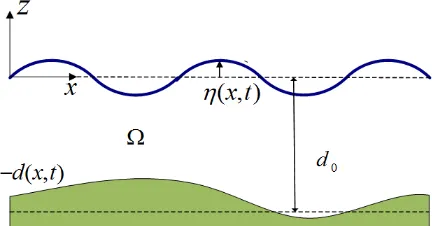
solution. Consider a layer of ideal fluid bounded below by a rigid bottom z =
−d(x, t) and above by free surface z =η(x, t), as depicted in Figure 1. We note
Figure 1. Schematic diagram of ideal fluid over a rigid bottom.
that to allow the bottom motion, we let it depends on timet. Under the assumption
of irrotational flow, mass conservation for incompressible fluid read as
φxx+φzz= 0 in Ω, (1)
whereφ(x, z, t) is the velocity potential. Along the free surface, kinematic boundary
condition and Bernoulli equation read as
φz=ηt+φxηx on z=η(x, t), (2)
φt+
1 2|∇φ|
2+gη= 0 on z=η(x, t). (3)
Along the bottom, kinematic boundary condition that corresponds to impermeable bottom is
S.S. Tjandra,
In the derivation of analytical solution, we neglect the non linear term in (2)-(4). Furthermore the boundary conditions are considered on the undeformed free surface
z= 0 and flat bottomz=−d0. The linearized equations are explicitly
φz=ηt on z= 0, (5)
φt+gη= 0 on z= 0, (6)
φz=−dt on z=−d0. (7)
Equations (5) and (6) are usually combined to yield
φtt+gφz= 0 on z= 0. (8)
The analytical solution for these problem given by equations (1),(6), (7) and (8) will be obtained by using integral transforms. We recall the definition of Laplace transform and its inverse as follows
¯
plane. Fourier transform and its inverse are defined as
˜
In paragraph below we describe the steps in getting the analytical solution. We
apply the Fourier transform w.r.txand the Laplace transform w.r.t. tfor equations
(1), (6), (7) and (8) to yield
General solution of the ordinary differential equation (9) is
˜ ¯
φ(k, z, s) =A(k, s) coshkz+B(k, s) sinhkz. (13)
In order to satisfy boundary condition (12), the relation between coefficientsAand
B should follow
B(k, s) =−s
2
gkA(k, s). (14)
In order to get the coefficientsAandB, we substitute (13) and (14) into equation
Solution (13) with coefficients (14) and (15) yield the following velocity potential in transformed variables
˜
Surface elevation in transformed variables can be obtained from (16) and (10) as follows
Next, applying the inverse Laplace and Fourier transforms of (17) to yield
η(x, t) = −1
In order to calculate (18) we must prescribe a specific bottom motion. For that purpose, we focus on a bed displacement governed by
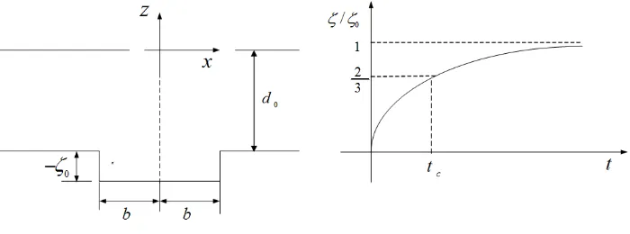
d(x, t) =d0−ζ0(1−e−αt)H(b2−x2), (19)
where H is the heaviside step function. This motion is illustrated in Figure 2, in
which the middle section of the bed−b < x < bis moved downward to a maximum
displacement ζ0 in an asymptotic manner, prescribed by (1−e−αt), in which α
is related to a characteristic timetc. A characteristic timetc is the time required
for the bottom to reach 2
3 of the maximum displacement. This type of bottom
motion is used in Hammack experimental works, as recorded in [1] and it is called
the exponential bottom motion. The choice of the ratio ζζ
0 = 2
3 is also used in [1].
Figure 2. Bed displacement model.
The bed displacement (19) is then applied to (18) by expressing the Fourier and Laplace transforms of it
S.S. Tjandra,
so that the surface elevation becomes
η(x, t) = −1 2π
Z ∞
−∞
−2ζ0sinkb
kcoshkd0
e−ikx
1
2πi Z
Γ
αsest
(s2+ω2)(s+α)ds
dk. (21)
In the next paragraph we give step by step of calculating the complex integral (21) using the residue theorem (see for reference [3] and [8]). We denote the integrand as f(s) = (s2+ωαs2)(s+α) which has three poles at s = ±iω and s = −α, see the
illustration in Figure 3.
Figure 3. Contours for the inverse Laplace transform.
LetCR andCL are semi circles on the right and left half respectively, of the
complexsplane. And sinceCR = Γ∪C1 and CL = Γ∪C2 as depicted in Figure
3, the complex integral in (21) can be evaluated as
Z
Γ
f(s)estds=
−H
CRf(s)e
stds+H
C1f(s)e
stds, fort <0,
H
CLf(s)e
stds−H
C2f(s)e
stds, fort >0. (22)
Note that by Jordan’s LemmaRC
1f(s)e
stdsandR
C2f(s)e
stdsare zero since
lim
s→∞|f(s)|= 0.
Furthermore, with Cauchy’s residue theorem, the integral (22) becomes
Z
Γ
f(s)estds=
0, fort <0,
2πiP3
j=1
Res s=s0j
with
The residue formula for a rational function at the simple poleiω,−iω, and−αwill
be used. HenceR
Γf(s)e
Finally, the inverse transform reads
1 Substituting (23) into (21) yield
η(x, t) = −ζ0
Take only the real part of the resulting integral, and note that ω follows from the
dispersion relation ω(k) =√gktanhkd0, moreover ω12cosωt and
1
ωsinωtare even
functions in k, hence we have the water surface displacement resulting from the
exponential bed motion as
η(x, t) = −2ζ0
This is the explicit formula depending on the parameter of exponential bottom motionb,α,d0 andζ0.
3. Numerical Integration Result
In this section, we use the analytical solution (25) to simulate free surface elevation as response of the downward bottom thrust. First, we note that analytical evaluation for the integral would be complicated, and it will be approximated by numerical integration. Let I denotes the integrand of (25). Integral in (25) is
improper for two reasons, the infinite upper boundary, and singularity atk= 0. To
handle this improper integral, we rewrite the integral (25) as R∞
0 Idk = R1
0 Idk+ R∞
1 Idk. We analyze each of these integrals and we choose the integral which
S.S. Tjandra,
We check the convergence ofR∞
1 Idk by first observe the following
|I| ≤ |coskx||sinkb|
Using comparison test with the convergent integral R∞
1
dk. Similar argument with the convergent integral
R∞
convergence of these components, yield the convergence ofR∞
1 Idk.
The convergence and value of this integral is also check by calculating its value
at a chosen position and time,x= 61 andt= 2, by means of trapezoidal numerical
integration. Their values are displayed in Table 1. For example, the first data in
Table 1 show R1.1
1 I(61,2)dk = 1.1034 .10
−6. It is shown in the right column,
the value ofR∞
1 Idk is close to zero, with accuracy up to 10
−6which suggest that
R∞
1 Idk≈0. We also check the value of this integral at others position and time.
Next, we focus on applying numerical integration for calculatingR1
0 Idk. To
handle the singularity of the integrand at k = 0 we first observe its limit value.
By L’Hopital’s rule limk→0I =b(e−αt−1). For numerical integration, we apply
the trapezoidal rule whereas the value of I at k= 0 is taken to be its limit value
b(e−αt−1). In Table 2 we calculateRb
aI(61,2)dkfor various integration interval in
[0,1]. For example, the first data in Table 2 showR0.1
0 I(61,2)dk=−0.49005716.
Finally, after analyze the integralR1∞IdkandR01Idk, we conclude that integral in
(25) can be approximated asR0∞Idk≈R1
0 Idk.
Table 1. CalculatingRb
aI(61,2)dkusing trapezoidal rule with4x=
Table 2. CalculatingRb
aI(61,2)dkusing trapezoidal rule with4x=
0.0001, for [a, b]⊂[0,1]
[a, b] Value
[0,0.1] -0.49005716 [0,0.2] -0.47260392 [0,0.5] -0.47393012 [0,0.6] -0.47383404 [0,0.7] -0.47393062 [0,0.8] -0.47391938
[0,1] -0.47391243
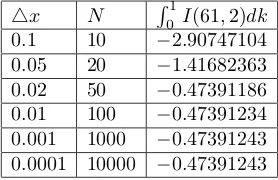
Next, we calculate η(61,2) as R01I(61,2)dk using various length of 4x as
shown in Table 3. We conclude that taking 4x = 0.0001 is enough to get the
correct result up to 10−5.
Table 3. Calculatingη(61,2)≈R1
0 I(61,2)dk using various length of4x.
4x N R1
0 I(61,2)dk
0.1 10 −2.90747104
0.05 20 −1.41682363
0.02 50 −0.47391186
0.01 100 −0.47391234
0.001 1000 −0.47391243
0.0001 10000 −0.47391243
In later calculations, we use integration interval [0,1] with4x= 0.001. Here,
we simulate surface wave generated by specific bottom motion. We use the
expo-nential bottom motion (19) with parameterd0= 5,b= 61 andζ0= 1. We choose
the characteristic time tc = 0.08. The explicit analytical formula (25) is defined
for t >0 and x∈ R presents the free surface elevation as an even function in x.
In Figure 4 we plot the snapshots of surface elevation on the half interval x > 0
for subsequent time t = 0.04, t = 0.1, t = 0.25, t = 0.5, t = 1 and t = 1.2 near
the characteristic time. The result shows the surface wave will increase correspond with bottom movement and after the characteristic time, it will form a negative leading wave.
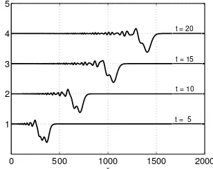
In Figure 5 we plot the snapshots of surface elevation on the half interval
x >0 for subsequent time t = 5, t= 10,t = 15 andt = 20 when bottom motion is complete. The result show that the free surface responds in terms of a negative leading wave, followed with dispersive train of waves. Moreover, we observe that
the maximum amplitude of the surface is 0.6 which is approximately half of the
bottom amplitudeζ0. And this follow the analytical prediction as described in [2].
S.S. Tjandra,
0 50 100 150 200 250 300
1 2 3 4 5 6 7
x
t=0.5 t=1 t=1.2
t=0.25
t=0.1
t=0.04
Figure 4. Snapshots of analytical surface elevation as response
of a downward bottom thrust, at the early stage of generation process.
0 500 1000 1500 2000
1 2 3 4 5
x
t = 20
t = 15
t = 10
t = 5
Figure 5. Snapshots of analytical surface elevation after
genera-tion being completed. The developed wave experiences only slight deformation during its evolution over flat bottom
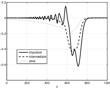
Further, we investigate the effect of characteristic timetc. The same bottom
motion and parameter are used, with difference only on the choice of the charac-teristic timetc. We use some different characteristic times,tc= 0.08,tc = 0.8, and
tc = 4.0, that represent three different kind of bottom motions: impulsive,
inter-mediate and slow motion, respectively. The results at t= 10 are plotted together
0 200 400 600 800 1000 −0.6
−0.4 −0.2 0 0.2
x impulsive intermediate slow
Figure 6. Surface wave profiles at time t = 10 for impulsive,
intermediate and slow bottom motions.
4. Concluding Remarks
We have presented the explicit analytical formulation of surface elevation as response of bottom motion in terms of improper integral. Analyzing the conver-gence of this integral, and applying trapezoidal numerical integration have given us the development of free surface wave. Simulation of the downward bottom thrust yields a negative leading wave, which is followed with a dispersive wave train. The explicit analytical formula allowing us to simulate transient wave for different type of motion. Among three types of motions: impulsive, intermediate, and slow, the impulsive motion yield the maximum amplitude of leading wave. In the case of im-pulsive bottom motion, the amplitude and velocity of our leading wave confirm the analytical formula. It should be noted that once the wave has been generated, our description does not considered topographic change during the evolution. So, for predicting wave characteristic at the beach, further investigations are still needed. Also, our analysis here was only for a downward bottom motion.
Acknowledgement. Financial support from Riset Desentralisasi ITB 2015,
311n/I1.C01/PL/2015 and 310c/I1.C01/PL/2015 are greatly acknowledged. Par-tial support from the Ensemble Estimation of Flood Risk in a Changing Climate project funded by The British Council through their Global Innovation Initiative are also acknowledged.
References
S.S. Tjandra,
[2] Hammack, J.L., ”A note on tsunami: their generation and propagation in an ocean of uniform depth”,J. Fluid Mech.,4(1973), 769-799.
[3] Mei, C.C., and Yue, D.P.,Advanced series on Ocean Engineering, World Scientific, 2005. [4] Dutykh, D., and Dias, F.Tsunami and non linear waves, Springer, 2007.
[5] Kervella, Y., Dutykh, D., and Dias, F., ”Comparison between three dimensional linear and non linear tsunami generation models”,Theor. Fluid Dyn.,21(2007), pp. 245-269. [6] Fuhrman, D.R., and Madsen, P.A., ”Tsunami generation, propagation, and run-up with a
high-order Boussinesq model”,Coastal Engineering,56(2009), pp. 747-758.
[7] Lynett, P., and Liu, P.L.F, ”A numerical study of submarine-landslide-generated waves and run-up”,Proc. R. Soc. Lond. A,458(2002), pp. 2885-2910.