A Multiple Lender Approach to Understanding
Supply and Search in the Equity Lending Market
ADAM C. KOLASINSKI, ADAM V. REED, and MATTHEW C. RINGGENBERG∗
ABSTRACT
Using unique data from 12 lenders, we examine how equity lending fees respond to demand shocks. We find that, when demand is moderate, fees are largely insensitive to demand shocks. However, at high demand levels, further increases in demand lead to significantly higher fees and the extent to which demand shocks impact fees is also related to search frictions in the loan market. Moreover, consistent with search mod-els, we find significant dispersion in loan fees, with this dispersion increasing in loan scarcity and search frictions. Our findings imply that search frictions significantly impact short selling costs.
SHORT SALE CONSTRAINTS MOTIVATEa large body of theoretical research in asset pricing. In addition, a growing body of empirical work confirms that these constraints have an economically meaningful impact.1Although this research
suggests that short sale constraints are important, relatively few empirical studies attempt to explain the variation of short sale constraints across stocks, and even fewer seek to provide a motivation for the origin of these constraints. Short sale constraints can take many forms, but one of the most important is the fee that short sellers pay to borrow shares in the equity lending market. Despite its one trillion dollar size, relatively little is known about this mar-ket because transactions are usually only visible to the two parties directly involved.2 Furthermore, the equity loan databases employed in the existing
∗University of Washington, University of North Carolina, and Washington University in St. Louis, respectively. The authors thank Robert Battalio, Darrell Duffie, Nicolae G ˆarleanu, Jennifer Huang, David Musto, Lasse Pedersen, an anonymous referee, the Editors, and semi-nar participants at the American Finance Association Conference, Barclays Global Investors, the Consortium for Financial Economics and Accounting Conference, the European Finance Associa-tion Conference, the IIROC-DeGroote Conference on Market Structure, Texas A&M, the University of Oregon’s Institutional Asset Management Conference, the University of Virginia, and the Uni-versity of Washington. We are grateful for financial support from the Q Group. Our data provider made this work possible and provided invaluable advice over the course of numerous discussions. Finally, we thank William Frohnhoefer for providing institutional details.
1The theoretical literature on short selling includesMiller (1977),Diamond and Verrecchia
(1987), andHong and Stein (1999), and empirical work demonstrating the significant economic
impact of short sale constraints includesGeczy, Musto, and Reed (2002),Ofek and Richardson
(2003),Asquith, Pathak, and Ritter (2005), andCao et al. (2008).
2Conversations with industry participants indicate that this is slowly changing. A central
counterparty exchange is slowly gaining volume (the exchange currently handles less than 1% of volume).
literature are provided by individual equity lenders, so researchers have not had an opportunity to draw conclusions about market-wide characteristics. As a result, a number of important questions remain unanswered: How much short selling can take place before borrowing shares becomes expensive? What causes borrowing to become expensive? What are the characteristics of the share lending supply curve? And, finally, how much variation in fees could a borrower expect to see across multiple lenders? We find that the answers to these questions are related to the presence of search frictions in the equity lending market.
The general dearth of empirical research on the equity lending market is inherently linked to its opacity, and one of the primary goals of this paper is to analyze the effects of this opacity. In one of the few theoretical models of the equity loan market,Duffie, G ˆarleanu, and Pedersen (2002, hereafter DGP) suggest that search frictions, which result from opacity, give share lenders market power, allowing them to charge fees to short sellers. We examine this model empirically in a number of ways. First, we find significant dispersion in loan fees, which is consistent with the existence of search frictions in the share loan market. In addition, using stock characteristics that DGP suggest as proxies for search frictions, we show that search frictions are related to loan fee dispersion. Finally, we find that loan fee dispersion sharply increases as the average loan fee moves from moderate to high levels, consistent with DGP’s hypothesis that search frictions are related to the costs of short selling. However, the relation between the average fee and the dispersion in fees is not monotonic: dispersion is also high when the average fee is abnormally low, resulting in a U-shaped pattern.
We also examine how search frictions allow lenders to change their prices in response to exogenous shifts in demand. In the existing literature, some con-troversy exists regarding the way demand affects prices; some researchers find that lending fees are unresponsive to increases in quantity (e.g.,Christoffersen et al. (2007)), whereas others find that large positive shifts in the demand for share loans can be manifested in increased lending fees (e.g.,Cohen, Diether, and Malloy (2007)). We resolve this apparent paradox by using a nonlinear two-stage least squares method to estimate the share loan supply schedule. We find that the loan supply schedule is essentially flat, and that specialness is invariant to quantity demand shocks most of the time. For example, for the average stock a movement from the 10th quantity percentile to the 90th results in a loan fee change of only five basis points. However, the slope of the supply schedule becomes positive and steep when demand shocks drive quantity to ab-normally high levels, consistent withCohen, Diether, and Malloy (2007).3For
example, a one standard deviation increase from the third to fourth standard
3Cohen, Diether, and Malloy’s (2007)results connect the demand for share loans to underlying
deviation of quantity is associated with a movement in abnormal loan fees from 3.2 basis points to 21.7 basis points.
To further investigate the relation between the supply curve and search fric-tions, we examine how the shape of the supply curve relates to several proxies for search frictions. We find evidence that the share loan supply schedule is steeper at high quantity levels when search costs are higher. In addition, we examine whether factors unrelated to search costs can explain the patterns in the data that we attribute to search costs. First, we find that variation in the types of lenders active in a particular stock’s loan market can explain some of the cross-lender dispersion in specialness. It is therefore likely that differ-ences in lender desirability are at least partly responsible for the dispersion we observe. However, our proxies for search costs continue to have a significant effect on dispersion even after controlling for variation in lender type. Second, we examine whether concentration in lender capacity, which could result in in-creased market power when quantity demanded is high, can explain our finding that supply curves tend to become steep at high quantity levels. However, con-trary to this hypothesis, we find that the loan supply curve is not statistically different between low and high levels of lender capacity concentration.
Our research has important policy implications. Because search frictions have a significant impact on lending fees, it follows that a reduction in these frictions would loosen short sale constraints. One way to reduce search fric-tions is to introduce a central clearinghouse for share loans, such as the NYSE lending post that was abandoned in the 1930s. Furthermore, there is evidence that short sale constraints reduce market efficiency (e.g., Asquith, Pathak, and Ritter (2005),Nagel (2005),Reed (2007), andCao et al. (2008)). Although some regulators and journalists accused short sellers of disrupting markets and reducing efficiency during the financial crisis of 2008, a large body of re-cent research suggests that market quality decreased after short sales were restricted in response to the crisis (e.g., Bris (2009), Boehmer, Jones, and Zhang (2009),Boulton and Braga-Alves (2010),Kolasinski, Reed, and Thornock (2013)). Taken together, these results suggest that centralizing the share loan market could potentially improve stock market efficiency. However, as Jones and Lamont (2002)document, some stocks became expensive to borrow even with a lending post. Further, we find other factors, in addition to search fric-tions, that can make borrowing expensive. Thus, although it is unlikely that a central clearinghouse would eliminate all borrowing difficulty in the share loan market, our evidence suggests that search frictions are a significant contributor to borrowing costs.
Finally, our findings also have broader implications for opaque financial mar-kets. The theoretical models we use to motivate our empirical tests need not be limited to the equity lending market. Insofar as their underlying assump-tions of agent heterogeneity, search fricassump-tions, and the lack of centralized price quoting are consistent with the institutional details of other over-the-counter markets, our results can be generalized to those contexts.
the equity lending market with a particular focus on the ability of search frictions to generate short sale constraints, and the resulting empirical impli-cations.Section IIdescribes the databases used in this study andSection III characterizes our findings.Section IVpresents our summary and conclusion.
I. Search Frictions and the Share Lending Market
A. Specialness, Search Frictions, and Price Dispersion
DGP present a dynamic model in which search frictions limit the frequency at which share lenders and borrowers are able to find one another. Thus, lenders, if they have some bargaining power, are able to charge a lending fee to short sellers that is equal to some fraction of the surplus short sellers believe they can gain. Short sellers are willing to pay the fee because, if they refuse, they might not be able to find another lender and thus would have to forgo their surplus. Over time, this lending fee declines to zero as short sellers drive down prices to their long-run equilibrium values. The magnitude of the lending fee, often termedspecialness, is increasing in lenders’ bargaining power, in frictions in the share lending market, and in demand for share loans.
In our investigation, we also draw on the industrial organization literature on search costs and price dispersion. When there is heterogeneity in seller costs, models in which buyers must search sequentially for a seller generally yield a positive relation between average prices, price dispersion across sellers, and search costs (Reinganum (1979), Sirri and Tufano (1998),Baye, Morgan, and Scholten (2006)). The DGP model does not predict dispersion in fees across lenders because it assumes no heterogeneity in lenders’ costs of providing share loans (DGP assume lenders’ costs are zero). However, in practice it is likely that some heterogeneity in lenders’ costs does exist, so if search frictions drive specialness, we would expect an increased average level of specialness to be associated with increased dispersion in specialness across lenders. Using data from multiple lenders, we compute dispersion in specialness across lenders for a given stock at a given point in time.4 We then examine the relation of this
dispersion to the average specialness in a given day, as well as investigate other proxies for search costs. InSection III.C,we explore the role played by alternative nonsearch explanations.
B. The Share Loan Supply Curve
Although search frictions are constant in the DGP model, they are not likely to be so in practice. As DGP point out, these frictions are likely to be close to zero
4One natural way to understand the DGP model in the context of heterogeneous search costs
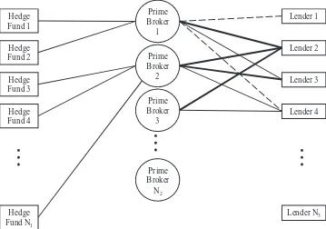
Hedge
Figure 1. Structure of the equity lending market. Figure 1 presents an example of the
structure of the equity lending market. Hedge funds, shown asHedge Fund 1throughHedge Fund N1, can be clients of multiple prime brokers,Prime Broker 1throughPrime Broker N2. These prime brokers can have relationships with multiple securities lenders,Lender 1throughLender N3. The relationships with these lenders can be regular (bold line), occasional (solid line), or infrequent (dashed line).
when demand for loans is low. In this case, brokers have more lenders than bor-rowers among their clients, so matching is nearly costless. In addition, brokers have the ability to contact different lenders for information about availability and pricing, and most of the time the lenders with whom they have an existing relationship have an ample supply of most stocks. However, conversations with industry participants indicate that certain stocks may not be available from all lenders, and in these cases we would expect brokers to search for shares. The existence of third-party lenders, or “finders” as inFabozzi (1997), supports this view.Figure 1shows the structure of these relationships.
The presence of fixed costs also likely lowers the number of willing lenders when demand is low, potentially giving these lenders some monopoly power. As share loan demand increases from very low to moderate levels, we expect the number of lenders to increase, thereby reducing monopoly power and yielding a downward slope in the left-hand portion of the share loan supply schedule.5
Moreover, the existing literature finds that loan rates tend to be lower for large loans than for small loans (D’Avolio (2002),Geczy, Musto, and Reed (2002)). In other words, the evidence suggests that volume discounting is prevalent in the equity lending market. Thus, we expect the share loan supply schedule to be nonmonotonic, with a downward slope at low quantity levels, a relatively flat slope for moderate quantities, and an upward slope at high quantity levels.
C. Alternative Explanations for an Upward Sloping Supply Curve and Loan Fee Dispersion
In addition to search costs, other economic factors could plausibly explain both dispersion in loan fees and an upward sloping share loan supply curve. We describe these alternative hypotheses below and analyze them empirically inSection III.C.
C.1. Differences in Lender Desirability
Because borrowers are able to borrow from multiple lenders, and because each lender draws from portfolios with different characteristics, it is reasonable to hypothesize that borrowers may prefer some lenders to others. Differences in lender desirability would lead to differences in the average fees charged by lenders. Similarly, differences in lender desirability could lead to price disper-sion, as borrowers pay more to borrow from certain lenders and less to borrow from others. We refer to this hypothesis as the lender desirability hypothesis.
C.2. Lender of Last Resort
Another possible explanation is that, for a given stock, there is a dominant lender who has a large proportion, but perhaps not all, of the lendable shares. Such a lender could act as the “lender of last resort.” When demand for share loans is low, the lender of last resort must compete with other lenders. However, because the competing lenders have a limited inventory, a sufficiently large demand shock could plausibly deplete this inventory, giving the lender of last resort a monopoly. As a result, we would expect a supply curve that is flat at low levels of quantity, where lenders compete, and then upward sloping once
5For example,Kaplan, Moskowitz, and Sensoy (2013)conduct an experiment in which they
quantity reaches the point at which the lender of last resort has monopoly power. If the lender of last resort hypothesis is true, the upward sloping supply curve is driven more by inventory concentration than by search costs.
C.3. Lender Cost Differences
In Duffie (1996), the supply curve of treasuries available for loan becomes steep and upward sloping not because of search costs, but because of differences in the cost of lending among potential lenders. Duffie refers to these costs as transactions costs, but they could just as easily be interpreted as costs that are constant for each lender and varying across lenders. Lenders with low costs provide loans in most scenarios, but lenders with high costs are only willing to lend when demand shocks drive loan fees to sufficiently high levels. In other words, the fact that we see an increase in the slope of the supply curve may be a result of differences in lenders’ costs, not search costs.
II. Data
To test the hypotheses developed above, we use databases from several different sources. Our principal analyses use two databases containing loan quantities and lending fees from 12 different equity lenders: the first contains transaction-level data over the period September 26, 2003 to May 9, 2007, and the second contains data at the stock-day level over the period September 26, 2003 to December 31, 2007. In a supplemental analysis, we also examine the quantity of shares available to be borrowed in the market over the period January 1, 2007 to December 31, 2009.
A. Loan Quantity and Lending Fees
The data provider for our study is both a market maker in the equity loan market and a data aggregator for major equity lenders. In its role as a market maker, the firm intermediates loans by borrowing from one party and lending to another. As such, our data provider also contributes its own transactions to the database. More importantly for the purposes of this paper, in its role as a data aggregator our data provider collects information about equity loan market conditions from several equity lenders. In particular, the firm provides current and historical stock loan market rates based on live data feeds from equity lenders. These lenders contribute current and historical data about their own loan portfolios in exchange for access to this market-wide information.
Our database consists of historical loan portfolios from 12 lenders. As shown inTable I, the lenders providing data are direct lenders, agent lenders, retail brokers, broker-dealers, and hedge funds.6The principal owners of the shares
6Despite the apparent distinction between lender types, our data provider has not provided
The
Journal
of
Finance
R
Equity Lending Database Statistics
Table Ipresents summary statistics for the transaction-level equity lending database, which covers September 26, 2003 to May 9, 2007 (for certain lenders coverage is a subset of this period).Percent of Obs.is the percentage of observations that each lender accounts for in the database.Rebate Rateis the rebate rate on cash collateral for securities on loan.Number of Relationshipsis the number of loans made in each stock on a daily basis for a given lender. The database is discussed in detail inSection IIof the text.
Rebate Rate Number of Relationships (in percent) (stock/day)
Lender Percent
ID Lender Type Description of Obs. Mean Median Mean Median Max
1 Broker-dealer Broker-dealers box to other broker-dealers, some lending to hedge funds
16.10% 1.63 1.55 2.84 1 225
2 Broker-dealer Retail brokerage accounts lent to broker-dealers
7.86% 2.65 1.50 1.27 1 26
3 Broker-dealer Broker-dealer box to other broker-dealers, conduit trades
6.85% 4.13 4.25 2.02 1 31
4 Direct lender Hedge fund assets lent directly to broker-dealers
0.07% 0.78 1.08 9.92 8 204
5 Broker-dealer Broker-dealers box to other broker-dealers, conduit trades
3.52% 2.47 2.00 1.25 1 39
6 Broker-dealer Broker-dealers box to other broker-dealers, some lending to hedge funds
31.39% 4.20 4.30 5.74 4 136
7 Broker-dealer Broker-dealers box to other broker-dealers, some lending to hedge funds
6.63% 2.53 1.75 5.06 2 232
8 Direct lender Mutual fund assets direct to broker-dealers 17.92% 3.19 3.15 1.87 1 102 9 Broker-dealer Hedge fund, pension plans assets lent
directly to other hedge funds or broker-dealers, some conduit trades
0.83% 4.60 5.15 3.27 2 40
10 Direct lender Hedge fund assets lent directly to broker-dealers
0.30% 2.58 1.00 1.01 1 2
11 Agent lender Endowments, pension plan assets lent to broker-dealers
4.95% 4.33 4.75 1.43 1 101
that are lent (both directly and through agents) are retail brokerages, pension plans, insurance companies, and mutual funds. These market participants represent 36% of the securities lenders by number.7 In most of the analyses
that follow, including the estimation of the supply schedule, we use the sum of outstanding share loans by all lenders normalized by total shares outstanding as our measure of market loan quantity.
We use two separate equity lending databases: the first database comprises 5,042,056 observations of individual loan transactions from September 26, 2003 to May 9, 2007 and includes the number of shares, the daily loan rate, and sev-eral identification variables. The loan rate is the interest paid on the borrower’s collateral, also known as the rebate rate. The relative scarcity of a particular stock is measured in terms of its specialness, or the difference between its loan rate and the market’s prevailing, or benchmark, loan rate. Our data provider computes specialness at the firm-day level and this variable is contained in the second database we use, which contains data that has been aggregated to the firm-day level. In addition to daily specialness, the aggregate database contains a measure of the daily quantity and several identification variables. It comprises 1,511,874 observations of loan transactions aggregated to the stock-day level over the period September 26, 2003 to December 31, 2007. We use this aggregate data in our analysis of the share loan supply curve (Tables IV–VI below).
As discussed above, the database of individual transactions contains the daily loan rate. To calculate the dispersion in loan fees (Tables VIIandVIIIbelow), we need a loan-specific measure of specialness. However, each lender may have a different benchmark rate. Based on D’Avolio (2002)and Geczy, Musto, and Reed (2002), we calculate specialness by taking the benchmark rate to be the federal funds rate minus a 10 to 20 basis point spread for each lender. We use the mode of the distribution of loan fees above the federal funds rate to identify each lender’s spread (the difference between the loan rate and the benchmark) by loan size category.8 The median spread is 16 basis points, and the spread
has a relatively large range: the 25th percentile is one basis point and the 75th percentile is 50 basis points. Among loans above $100,000, the interquartile range is 0 to 25 basis points.
B. Lender Relationships
We also examine the extent to which lenders have relationships with mul-tiple borrowers. For each stock on each day, we count the number of trans-actions made by a given lender. Because borrowers consolidate orders to take advantage of volume discounts and thereby minimize transaction costs, each
7State Street’s publicly available white paper, “Securities Lending, Liquidity, and Capital
Market-Based Finance,” indicates that there were 33 dealers in the equity lending market as of 2001.
8As inD’Avolio (2002) and Geczy, Musto, and Reed (2002), loans are categorized as small
transaction in a given stock on a given day is likely to represent a unique bor-rower. The number of transactions for each lender therefore serves as a proxy for the number of unique borrowers, or “relationships,” that a lender has on a given day.
InTable I, we report descriptive statistics on the time series of each lender’s relationships. Interestingly, we find significant variation across lenders in the mean number of relationships, with the average number of relationships per day ranging between one and 10. Furthermore, there is a dynamic aspect to the number of relationships: the mean and median are well below the maximum for most firms. To take one example, for lender #7 the maximum number of relationships is 232, but the mean number of relationships is only 5.06 and the median is 2. The disparity we find between the maximum versus the means and medians indicates that the number of relationships is not constant, which is consistent with the idea that borrowers choose to search for stocks only when the costs of searching are exceeded by the benefits of finding loans. Intuitively, this could mean that borrowers have a few relationships with lenders from whom they borrow the majority of their shares, but for scarce stocks borrow-ers search across a large number of potential lendborrow-ers. We also note that the cross-sectional variation in the number of relationships documented here is consistent with heterogeneity in search costs.
C. Data Compilation
For our analysis of the share loan supply curve, we use the aggregate database, which contains 1,511,874 daily observations on loan fees and quan-tities. To this data set we add the daily stock price, ask price, bid price, and shares outstanding for each firm using data from the Center for Research in Security Prices (CRSP). We also addFederal Funds Rate, which is the effective federal funds rate from the H.15 statistical release provided by the Federal Reserve;S&P Price/Earnings,which is defined as the monthly price to earn-ings ratio for the S&P500 from Compustat; andVIX, which is calculated as the rolling mean value of the CBOE volatility index for the S&P500 over the preceding 22 trading days.
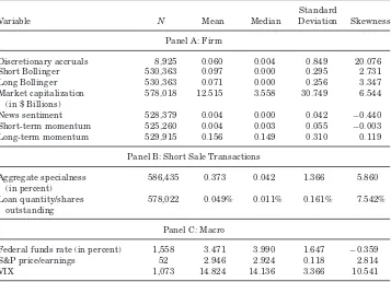
We winsorize all variables in the aggregate database at the 1st and 99th percentiles and we filter our database to include only those firms with at least 250 observations. After this filter is applied, 586,435 observations remain in the database. In Table II we report summary statistics for the final sample. Although the average value of Specialness is only 37 basis points, it has a standard deviation of 1.36 and it is highly right-skewed, with a skewness of 5.86. In addition,Loan Quantityas a percentage of shares outstanding is also highly right skewed.
III. Results
Table II
Summary Statistics of Instruments and Short Sale Variables
Table IIcontains summary statistics for the aggregate-level database, which contains 586,435
observations at the firm-day level for the period September 26, 2003 to December 31, 2007. The database is filtered to include only those firms with more than 250 observations.Discretionary Accrualsis calculated quarterly as inSloan (1996).Short(Long)Bollingeris an indicator variable that takes the value one if a stock’s price is more than two standard deviations above (below) the 20-day moving average price and zero otherwise.Market Capitalization, in billions, is from CRSP.
News Sentimentis a numerical score based on textual analysis of publicly released firm-specific news articles, where low (high) scores indicate negative (positive) news.Short-Term Momentumis the raw buy-and-hold return of a stock over the previous five trading days andLong-Term Momen-tumis the one-year momentum factor as inCarhart (1997).Loan Quantity / Shares Outstanding
is the quantity of shares borrowed divided by the number of shares outstanding each day for each firm.Specialness, in percent, is a measure of the cost of borrowing a stock and is calculated as the difference between the rebate rate for a specific loan and the prevailing market rebate rate.Federal Funds Rateis the effective rate available in the H.15 statistical release from the Federal Reserve.
S&P Price/Earningsis the monthly price to earnings ratio for the S&P500 from Compustat.VIXis the rolling mean value of the CBOE volatility index for the S&P500 over the preceding 22 trading days. All variables are winsorized at the 1st and 99th percentiles.
Standard
Variable N Mean Median Deviation Skewness
Panel A: Firm
Discretionary accruals 8,925 0.060 0.004 0.849 20.076
Short Bollinger 530,363 0.097 0.000 0.295 2.731
Long Bollinger 530,363 0.071 0.000 0.256 3.347
Market capitalization (in $ Billions)
578,018 12.515 3.558 30.749 6.544
News sentiment 528,379 0.004 0.000 0.042 −0.440
Short-term momentum 525,260 0.004 0.003 0.055 −0.003
Long-term momentum 529,915 0.156 0.149 0.310 0.119
Panel B: Short Sale Transactions
Aggregate specialness (in percent)
586,435 0.373 0.042 1.366 5.860
Loan quantity/shares outstanding
578,022 0.049% 0.011% 0.161% 7.542%
Panel C: Macro
Federal funds rate (in percent) 1,558 3.471 3.990 1.647 −0.359
S&P price/earnings 52 2.946 2.924 0.118 2.814
VIX 1,073 14.824 14.136 3.366 10.541
0.78 0.83 0.88 0.93 0.98 1.03 1.08
1 2 3 4 5 6 7 8 9 10
Speci
a
lnes
s
Trade Quantity / Outstanding Shares (grouped into deciles)
Mean 95% Confidence Interval
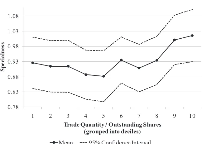
Figure 2. Specialness as a function of trade quantity in 2006.Trade quantity is divided by outstanding shares to account for persistent differences in loan quantities across securities. For each firm, these relative quantities are then assigned to a decile based on their position relative to other trade quantities for that firm and year. The figure plots the mean specialness across all firms for each decile. Specialness, in percent, is a measure of the cost of borrowing a stock and is calculated as the difference between the rebate rate for a specific loan and the prevailing market rebate rate. The rebate rate for an equity loan is the rate at which interest on collateral is rebated back to the borrower.
A. Modeling the Share Loan Supply Curve
Presumably, short sale constraints arise as short sellers’ demand for share loans increases.9 However, not all increases in share loan demand lead to
increases in loan fees (Christoffersen et al. (2007)). So the question remains, by how much does demand need to increase before loan fees increase?
As a first pass, in Figure 2 we conduct a simple experiment, modeled on that ofD’Avolio (2002), in which we plot specialness (or excess loan fee) as a function of quantity loaned. To account for persistent differences in loan quan-tity across securities, we calculate relative quantity loaned. In other words, quantity is measured as the rank of normalized loan quantity, defined as the number of shares lent divided by total shares outstanding. We find that spe-cialness declines mildly in loan quantity at low levels of loan quantity, but when loan quantity is above the 70th percentile, specialness increases sharply in loan quantity. The changing sensitivity of specialness to quantity has prac-tical importance for borrowers: upward shifts in the quantity demanded do not necessarily increase loan prices and may even decrease them in some cases.
This initial approach is inherently limited, however. The supply schedule cannot be mapped out correctly using prices and quantities unless the supply curve does not shift during the measurement period. To trace out the supply curve more carefully, we turn to a two-stage regression approach, similar to that of Angrist, Graddy, and Imbens (2000). Specifically, we use exogenous shifts in the demand for equity loans as a means to identify the supply curve. As discussed inSection I.B, economic theory suggests that the share loan supply curve may not be linear. To allow for this possibility, we employ a nonlinear technique that builds on the linear approach of Angrist, Graddy, and Imbens (2000).
InSubsection A.1below, we use economic theory to propose several instru-ments for share loan demand and then conduct an empirical falsification test of their validity. InSubsection A.2we describe our technique for estimating the share loan supply curve and we present our results. Finally, inSubsection A.3, we examine how the shape of the supply curve differs for firms with different search cost characteristics.
A.1. Instruments for Share Loan Demand
To identify the share loan supply schedule, we must use variables that affect the demand for loans but not the supply. Prior research suggests that most of the supply of shares available for loan comes from institutions with stable, low-turnover portfolios (e.g.,D’Avolio (2002)). On the other hand, the literature has shown that many short sellers have relatively short time horizons.10Thus,
one category of potentially valid instruments includes variables that are re-lated to short-term trading strategies but not long-term trading strategies. It stands to reason that low-turnover institutions are, by definition, not concerned with the shorter term components of price movements. Accordingly, variables that isolate the short-term components of price fluctuations are likely to make valid instruments, consistent withBoehmer, Jones, and Zhang’s (2008, p. 498) finding that “. . .short selling is dominated by short-term trading strategies.” Accordingly, in what follows below we define and discuss five candidate in-struments that are likely to affect the demand for loans but not the supply:
News Sentiment,Short-Term Momentum, Short Bollinger,Long Bollinger,and
Discretionary Accruals.
One variable that is likely to impact the strategies of short sellers but not the strategies of low-turnover institutions is dailyNews Sentiment, which is a measure of the amount of positive or negative information contained in pub-licly released firm-specific news articles. Low-turnover institutions (i.e., equity lenders) are unlikely to trade every time there is a news article about one of the stocks in their portfolio. On the other hand,Engelberg, Reed, and Ringgen-berg (2012) and Fox, Glosten, and Tetlock (2010)show that short sellers do respond to daily news events. Accordingly, we consider News Sentiment as
10Geczy, Musto, and Reed (2002)show that the median duration of a stock loan is three trading
a potential instrument for share lending demand, where News Sentiment is defined for each firm and day as a numerical score between −1 and 1; low scores indicate negative news and high scores indicate positive news. The news data come from RavenPack, Inc., a leading provider of news analytics data for use in quantitative and algorithmic trading. In the normal course of its busi-ness, RavenPack uses proprietary algorithms to process news articles and press releases into machine-readable content and the data used in this study are de-rived from all news articles and press releases that appeared in the Dow Jones newswire, which includes, among other sources, the Wall Street Journaland Barron’s.
We also consider variables that capture the short-term component of price fluctuations. Specifically, we consider several variables related to technical analysis. Survey evidence suggests that institutional portfolio managers use technical trading rules when their time horizons are short (weeks), but not when their time horizons are long (e.g.,Carter and Van Auken (1990),Menkhoff (2010)). Accordingly, we consider Short-Term Momentum as an instrument, where Short-Term Momentum is defined as the raw buy-and-hold return of a stock over the previous five trading days. Diether, Lee, and Werner (2010) show that short sellers do respond to short-term momentum; however, it is unlikely that low-turnover institutions, which provide the bulk of lendable shares, respond to it. To make sure our short-term measures of returns are isolating the high-frequency component of price movement, we also include
Long-Term Momentumas a control variable, where Long-Term Momentumis
defined as the traditional one-year momentum factor as inCarhart (1997). In addition, we use another technical trading rule, namely, Bollinger bands (Bollinger (2002)), to motivate two additional candidate instruments. Specifi-cally, the Bollinger band strategy prescribes going short and long when a stock price is respectively above or below its 20-day moving average by more than two standard deviations.11We use the rule to define the indicator variables Short
BollingerandLong Bollinger, whereShort BollingerandLong Bollingerequal
one when a stock is respectively above or below its 20-day moving average by more than two standard deviations and zero otherwise.
Finally, we considerDiscretionary Accruals, as computed inSloan (1996), as a potential instrument. Discretionary accruals constitute a decision by man-agement to shift earnings from one period to another. Thus, high or low dis-cretionary accruals cannot persist and must, by construction, be followed by a reversal. Recent accounting studies suggest that this reversal occurs in less than a year, and all the negative (positive) abnormal returns associated with high (low) discretionary accruals are realized by the time of the accrual re-versal (e.g., Allen, Larson, and Sloan (2010), Fedyk, Singer, and Sougiannis (2011)). Discretionary accruals are therefore unlikely to be related to trading by low-turnover institutions and hence the quantity of lendable shares. On the other hand, prior literature finds that short selling is related to discretionary accruals (e.g.,Cao et al. (2008)).
11Technical traders differ on the precise parameters, so we choose a 20-day moving average and
Having made an a priori case for our instruments based on economic theory, we next conduct a formal empirical falsification test of their validity. For this test, we use a data set that contains the aggregate number of shares that equity lenders have available for loan over the period January 1, 2007 to December 31, 2009. We then test whether any of our instruments are significantly related to this aggregate quantity of lendable shares. If they are not, we infer that our instruments meet the exclusion restriction and are unrelated to the quantity of lendable shares.
The data we use for this test comes from Data Explorers, a leading provider of data in the equity loan market. Data Explorers aggregates and distributes information regarding the equity lending market at the daily frequency. The data are sourced directly from a wide variety of contributing customers in-cluding beneficial owners, hedge funds, investment banks, lending agents, and prime brokers. The database contains information on the aggregate quantity lenders actually lend out as well as the aggregate quantity of shares lenders
haveavailablefor loan, including those not lent. Our falsification test uses the
quantity available normalized by shares outstanding. We henceforth refer to this variable as lendable shares.
To conduct our falsification test, we run the following panel data regression in which the dependent variable is the log of the number of lendable shares and the independent variables are the candidate instruments discussed above:
Lendable Sharesit= β1Accrualsit+β2ShortBit+β3LongBit+β4Newsit
+β5STMomit+Controlsit+FEi+εit,
(1)
where Accrualsare discretionary accruals, ShortB and LongB are the short and long Bollinger indicator variables,Newsis news sentiment, andSTMom is short-term momentum. We include stock fixed effects, and we cluster the standard errors by stock and day to ensure robustness to heteroskedasticity as well as serial and cross-sectional correlation. If the candidate instruments meet the exclusion restriction, they should have no explanatory power in this regression. The results, presented in Table III, are consistent with our a pri-ori arguments. The coefficients on our candidate instruments (Discretionary
Accruals, Short Bollinger, Long Bollinger, News Sentiment, and Short-Term
Momentum) are individually and jointly statistically indistinguishable from zero.
In addition to being statistically insignificant, our point estimates suggest that the effect of our candidate instruments on lendable shares is also econom-ically negligible. Take, for instance, the coefficient estimate onNews Sentiment of−0.0129. This implies that a one standard deviation increase inNews
Sen-timentof 0.042 units shifts the log of lendable shares by−0.0005 [−0.0005=
Table III
Effect of Candidate Instrumental Variables on the Quantity of Lendable Shares
Table III displays the results of a panel data regression ofLendable Shares on five different
candidate instruments for the period January 1, 2007 to December 31, 2009 of the form
Lendable Sharesit=β1Accrualsit+β2ShortBit+β3LongBit+β4Newsit
+β5STMomit+Controls+FEi+εit.
Lendable Sharesis the natural log of the number of shares available for loan each firm and day as a percentage of shares outstanding. The candidate instruments are described in detail inSection
III.Aof the text.Federal Funds Rateis the effective federal funds rate as reported by the H.15
statistical release,Long-Term Momentumis the natural log of the one-year momentum factor as inCarhart (1997), S&P Price/Earningsis the natural log of the S&P500 price to earnings ratio for the preceding month, andVIX is the rolling mean value of the CBOE volatility index for the S&P500 over the preceding 22 trading days. Firm fixed effects are included andF-Test of Instrumentsassesses whether the candidate instruments are jointly different from zero. Robust standard errors clustered by firm and date are below the parameter estimates in parentheses. ∗∗∗indicates significance at the 1% level,∗∗indicates significance at the 5% level, and∗indicates significance at the 10% level.
Explanatory Variable Dependent Variable: Lendable Shares
Discretionary accruals 0.0002
(0.02)
Short Bollinger −0.0012
(0.00)
Long Bollinger 0.0032
(0.00)
News sentiment −0.0129
(0.02)
Short-term momentum −0.0125
(0.02)
Federal funds rate −0.0097
(0.01)
Long-term momentum 0.0232∗∗
(0.01)
S&P price/earnings −0.0387∗∗∗
(0.01)
VIX −0.0005
(0.00)
Firm fixed effect Yes
N 642,134
F-test of instruments 2.02
P-value 0.85
R2 0.02
News Sentiment, andShort-Term Momentumas instruments in the estimation of the supply curve.
A.2. Estimating the Share Loan Supply Schedule
Using the instruments discussed above, we estimate the share loan supply curve, which allows us to determine the influence of short sellers’ demand for share loans on specialness and the extent to which increases in loan prices are related to search frictions. We discuss our estimation procedure in detail below. To ensure comparability across stocks, we standardize our loan quantity vari-able. First, we divide quantity by total shares outstanding for each stock. This removes the effect of stock price on quantity, which would likely be sufficient for an estimation using market-wide quantity. However, because our lenders hold only a segment of the quantity of lendable shares of each stock, and because that segment may vary by stock, we need to further normalize each stock’s quantity. Thus, we standardize each stock’s quantity variable by subtracting the mean and dividing by the standard deviation of each stock’s loan quantity as a percentage of shares outstanding. We denote this standardized value of share loan quantity byQ.
Next, we need to take into consideration the highly skewed nature of both quantity and specialness, as well as the probable nonlinearity of the supply curve. To this end, we employ a trans-log specification in which we model the started natural log of specialness as a function of the started natural log of quantity demanded and its square.12 Greene (1997) notes that this sort of
specification is highly flexible and can be interpreted as a second-order ap-proximation of virtually any smooth functional form. Using the instruments discussed above, we thus represent the share loan demand and supply sched-ules as the following limited information system, with the supply schedule (3) as the identified equation:
LN(Qit+C)=δi+γ1LN(Sit+D)+γ2Accrualsit+γ3ShortBit+γ4LongBit
+γ5Newsit+γ6STMomit+Controlsit+ηit
(2)
LN(Sit+D)=αi+β1LN(Qit+C)+β2LN(Qit+C)2+Controlsit+εit, (3)
whereCandDare “start” constants that ensure the log is defined,13Qis loan
quantity, S is specialness, Accruals are Discretionary Accruals, ShortB and
LongB are the Short and Long Bollinger indicator variables, News is News
Sentiment, and STMom isShort-Term Momentum, all as defined above. The
Controlsvector includes the federal funds rate, long-term (365 day) momentum,
the level of the VIX index, and the P/E ratio of the S&P500. We also employ
12Since our quantity variable is standardized to make it comparable across stocks, it can take
negative values. Likewise, specialness can be negative. Therefore, asFox (1997)suggests for right-skewed variables with negative values, we use thestarted logtransformation of both quantity and specialness. Our results are not sensitive to the choice of start constant.
Table IV
First-Stage Estimation of the Share Loan Supply Curve
Table IVpresents the first-stage results from a two-stage instrumental variables panel data
re-gression of daily data over the period September 26, 2003 to December 31, 2007. The excluded instruments are discussed inSection III.Aof the text and, because there are two endogenous re-gressors (the started log quantity and its square), there are two first-stage regressions. Firm fixed effects are included in all models. TheF-statistic tests the null of weak identification. Robust stan-dard errors clustered by firm and date are shown below the parameter estimates in parentheses. ∗∗∗indicates significance at the 1% level,∗∗indicates significance at the 5% level, and∗indicates significance at the 10% level.
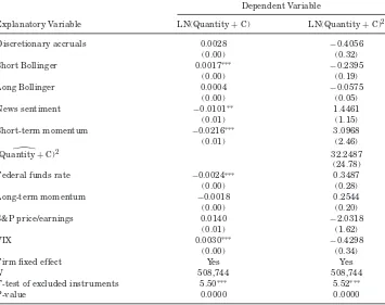
Dependent Variable
Explanatory Variable LN(Quantity+C) LN(Quantity+C)2
Discretionary accruals 0.0028 −0.4056
(0.00) (0.32)
Short Bollinger 0.0017∗∗∗ −0.2395
(0.00) (0.19)
Long Bollinger 0.0004 −0.0575
(0.00) (0.05)
News sentiment −0.0101∗∗ 1.4461
(0.01) (1.15)
Short-term momentum −0.0216∗∗∗ 3.0968
(0.01) (2.46)
(Quantity+C)2 32.2487
(24.78)
Federal funds rate −0.0024∗∗∗ 0.3487
(0.00) (0.28)
Long-term momentum −0.0018 0.2544
(0.00) (0.20)
S&P price/earnings 0.0140 −2.0318
(0.01) (1.62)
VIX 0.0030∗∗∗ −0.4298
(0.00) (0.34)
Firm fixed effect Yes Yes
N 508,744 508,744
F-test of excluded instruments 5.50∗∗∗ 5.52∗∗∗
P-value 0.0000 0.0000
stock fixed effects. We estimate equation (3) for a panel of stock-days over the period September 26, 2003 to December 31, 2007 using the nonlinear two-stage least squares procedure suggested byWooldridge (2002).14For robustness, we
also estimate the equation using limited-information maximum likelihood and Fuller-kmethods. The results from the first-stage regression, including a test of weak identification, are reported inTable IV. Our results from estimating equation (3), the supply curve, along with additional specification tests, are presented inTable V.
14We stress that we are not running whatWooldridge (2002, p. 236–237) calls “the forbidden
Table V
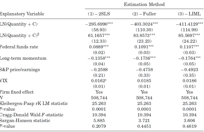
Second-Stage Estimation of the Share Loan Supply Curve.
Table Vpresents the second-stage results from a panel data regression of the started natural log of
loan fee (Specialness+D), on the started natural log of quantity (Q+C), according to the model:
LN(Specialnessi,t+D)=β1LN(Qi,t+C)+β2LN(Qi,t+C)
Table IV. Results below useC=10 andD=1, but are unchanged if we use other start constants.
Federal Funds Rateis the effective federal funds rate as reported by the H.15 statistical release,
Long-Term Momentumis the natural log of the one-year momentum factor as inCarhart (1997),
S&P Price/Earningsis the natural log of the S&P500 price to earnings ratio for the preceding month, andVIXis the rolling mean value of the CBOE volatility index for the S&P500 over the preceding 22 trading days. All variables are measured over the period September 26, 2003 to December 31, 2007. Firm fixed effects are included in all models and estimation is done using three different estimators (2SLS, Fuller, and LIML). Robust standard errors clustered by firm and date are shown below the parameter estimates in parentheses.∗∗∗indicates significance at the 1% level,∗∗indicates significance at the 5% level, and∗indicates significance at the 10% level.
Estimation Method
Explanatory Variable (1) – 2SLS (2) – Fuller (3) – LIML
LN(Quantity+C) −295.6990∗∗∗ −403.3024∗∗∗ −411.4129∗∗∗
(58.93) (110.30) (114.98)
LN(Quantity+C)2 61.1657∗∗∗ 83.8573∗∗∗ 85.5697∗∗∗
(12.33) (23.23) (24.22)
Federal funds rate 0.0889∗∗∗ 0.1091∗∗∗ 0.1107∗∗∗
(0.02) (0.03) (0.03)
Long-term momentum −0.1358∗∗∗ −0.1736∗∗∗ −0.1764∗∗∗
(0.04) (0.05) (0.05)
S&P price/earnings −0.2588 −0.4758 −0.4923
(0.21) (0.33) (0.35)
VIX 0.0162∗ 0.0185 0.0186
(0.01) (0.01) (0.01)
Firm fixed effect Yes Yes Yes
N 508,744 508,744 508,744
Kleibergen-Paap rK LM statistic 25.263 25.263 25.263
P-value 0.0001 0.0001 0.0001
Cragg-Donald WaldF-statistic 10.394 10.394 10.394
Sargan-Hansen statistic 5.885 3.721 3.606
P-value 0.2079 0.4451 0.4619
As can be seen in Table V, the log of quantity and its square are strongly significant in all specifications, implying that exogenous shifts in quantity de-manded impact specialness. Note that the parameters are qualitatively simi-lar across the three different estimation methods. Moreover, the specifications tests shown in Tables IVandVindicate that our instruments satisfy the ex-clusion restrictions and that weak instrument bias is not a concern.
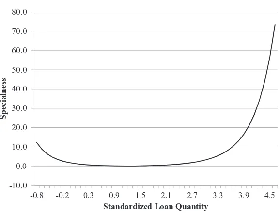
-10.0 0.0 10.0 20.0 30.0 40.0 50.0 60.0 70.0 80.0
-0.8 -0.2 0.3 0.9 1.5 2.1 2.7 3.3 3.9 4.5
Specialness
Standardized Loan Quantity
Figure 3. The share loan supply curve.Figure 3shows the price of borrowing a share ( Spe-cialness) as a function of the quantity (Standardized Loan Quantity) using the coefficient estimates shown inTable V.Standardized Loan Quantityis the quantity of shares borrowed divided by the number of shares outstanding, demeaned and normalized by the standard deviation to account for persistent differences in loan quantities across securities.Specialness, in basis points, is a measure of the cost of borrowing a stock and is calculated as the difference between the rebate rate for a specific loan and the prevailing market rebate rate. The rebate rate for an equity loan is the rate at which interest on collateral is rebated back to the borrower. Details on the supply curve estimation technique are presented inSection III.Aof the text. The figure displays the results from a 2SLS regression of LN(Specialness+D) as a function of LN(Standardized Loan Quantity+C), where
CandDare start constants suggested byFox (1997)to ensure the LN function is defined for all observations. Results are shown forC=10 andD=1, but the results are not sensitive to start constant values. We retransform the estimates to displaySpecialnessas a function of Standard-ized Loan Quantity. The figure is plotted between the 1st and the 99th percentiles ofStandardized Loan Quantity.
A.3. Cross-Sectional Patterns in Supply Curves
Given our findings above about the shape of the share loan supply curve, we next examine the importance of search costs in determining the supply curve’s shape. Specifically, we compare the shape of the supply curve for subsamples of stocks likely to have different search costs. DGP suggest that search costs are likely to be higher for small firms and illiquid firms, so we useMarket
Cap-italization andBid-Ask Spread, both calculated using daily data from CRSP,
as two of the measures on which we create subsamples. Interestingly, firm size and liquidity may also affect the shape of the supply curve under alternative explanations, so these two variables do not provide sharp distinctions between possible explanations.
We also use two search cost proxies related to the structure of the equity lending market that take advantage of the richness of our multiple lender data set. If finding lenders is costly, and smaller lenders are more difficult to find than large lenders, we expect search costs to be higher in equity loan markets that tend to be fragmented among many small lenders. Unlike size and liquidity, these proxies give us more traction in distinguishing various possible explanations, which we more fully discuss inSection III.C.
The first of our market structure–related search cost proxies is based on loan volume concentration. In the DGP model, agents are randomly matched with search intensityλand, all else equal, a lower search intensity leads to higher loan fees because it is more costly for agents to match. In practice, if the loan market is highly fragmented and no lender holds a significant amount of shares, it is likely that matching will be costlier. Accordingly, for each stock and each week, we compute the total loan volume for each lender as a fraction of shares outstanding and we use this measure to compute a Herfindahl index.15 Next
we compute the time-series average of this index for a given stock and refer to it as Lender Volume Concentration. Small values of this variable indicate that, for a typical week, lending in a given stock tends to be disbursed among many lenders with low volume, suggesting the market tends to be fragmented among many lenders with low levels of volume. If search costs are important in this market, and search costs play a role in shaping the supply curve, then we expect low values ofLender Volume Concentrationto be associated with higher supply curve slope coefficients.
Our second market structure–related search cost proxy is based on the num-ber of lenders active in a stock on a typical week as well as a proxy for lender size. To construct this measure, for each stock we compute the time-series average loan size of each lender (as a percentage of shares outstanding) and compare it to the average loan size across all lenders in the stock. If a lender’s average loan size is smaller than the average for all lenders in the stock, we refer to that lender as “small.” Otherwise the lender is “large.” Next, for each stock week, we count the number of small and large lenders and take the time-series averages for the stock and label these averages as Number Small
15We compute the index by week instead of by day because some stocks have many days for
LendersandNumber Large Lenders,respectively. The number of small lenders thus measures the extent to which a stock’s share loan market tends to be fragmented among many lenders with smaller-than-average volume. If search costs play an important role in shaping the supply curve, we expect the slope of the curve to be larger whenNumber Small Lendersis higher. On the other hand, if large lenders are easier to find, we expect search costs to be lower when
Number Large Lendersis high.
To test whether the shape of the supply curve is different for firms with dif-ferent search cost characteristics, we compute the sample medians of Market
Capitalization,Bid-Ask Spread, Lender Volume Concentration,Number Small
Lenders, andNumber Large Lenders. For each of these characteristics, we then
create two subsamples of stocks: low and high, where the low (high) subsample includes all firms with values below (above) the median of the relevant charac-teristic. We then reestimate the supply curve, allowing its parameters to differ across subsamples, and then conduct Wald tests of the null hypothesis that they do not differ.
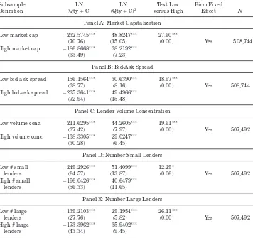
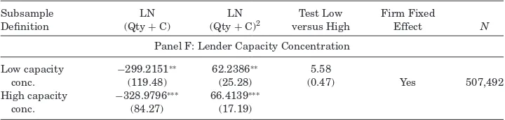
The results are reported inTable VI . We find that the parameters of the supply curve are statistically different for all measures of search costs,
includ-ingMarket Capitalization, Bid-Ask Spread, Lender Volume Concentration, as
well asNumber Small Lenders, andNumber Large Lenders. Consistent with the search cost hypothesis, we find that the coefficient on the quantity squared term is larger, and hence the supply curve is more steeply upward sloping, when firms are smaller, when firms are less liquid, and when firms’ loan vol-ume is dispersed among many lenders. Interestingly, whereas the results in Panels A, B, and C strongly support the search cost hypothesis, the results in Panels C and D are generally weaker. For bothNumber Small Lendersand Number Large Lenders, the curves are economically similar across subsamples. Thus, the results in Table VI generally support the search cost hypothesis, though not all search cost proxies appear to influence the shape of the supply curve.
B. Industrial Organization, Search Costs, and the Equity Loan Market
Table VI
Sensitivity of Share Loan Supply Curve to Firm Characteristics and Search Cost Proxies
Table VIpresents second stage results from six different panel data regressions that estimate the
share loan supply curve. In each panel, we examine the impact that a firm characteristic has on the supply curve by creating two subsamples of stocks, low and high, where the low (high) subsamples include all firms with values below (above) the median value of the relevant firm characteristic. We then jointly estimate the supply curve for the low and high subsamples, allowing the parameters to differ across subsamples, and conduct a Wald test of the null that the subsamples do not differ. The table displays the results for the LN(Quantity+C) and LN(Quantity+C)2parameters for the
low and high firm characteristic subsamples.Market Capis the average market capitalization for each firm from CRSP.Bid-Ask Spreadis the average bid-ask spread for each stock calculated using the closing mid-price on each day.Volume Concentrationis a Herfindahl index using each lender’s daily volume in a stock.# Small(Large)Lendersis the mean number of small (large) lenders that dealt in a particular stock each week.Capacity Concentrationis a Herfindahl index using each lender’s maximum possible loan volume in a stock. Robust standard errors clustered by firm and date are shown below the parameter estimates in parentheses.∗∗∗indicates significance at the 1% level,∗∗indicates significance at the 5% level, and∗indicates significance at the 10% level.
Subsample LN LN Test Low Firm Fixed
Definition (Qty+C) (Qty+C)2 versus High Effect N
Panel A: Market Capitalization
Low market cap −232.5745∗∗∗ 48.8247∗∗∗ 27.60∗∗∗
(70.76) (15.05) (0.00) Yes 508,744
High market cap −186.8668∗∗∗ 38.2192∗∗∗
(33.49) (7.23)
Panel B: Bid-Ask Spread
Low bid-ask spread −156.1564∗∗∗ 30.6390∗∗∗ 18.97∗∗∗
(38.77) (8.16) (0.00) Yes 508,744
High bid-ask spread −235.3641∗∗∗ 49.4966∗∗∗
(72.94) (15.48)
Panel C: Lender Volume Concentration
Low volume conc. −211.6295∗∗∗ 44.2605∗∗∗ 19.61∗∗∗
(37.42) (7.97) (0.00) Yes 507,492
High volume conc. −138.3305∗∗∗ 29.0247∗∗∗
(30.28) (6.45)
Panel D: Number Small Lenders
Low # small −249.2926∗∗∗ 51.4099∗∗∗ 12.29∗
lenders (64.57) (13.87) (0.06) Yes 507,492
High # small −196.0426∗∗∗ 40.6479∗∗∗
lenders (56.33) (11.65)
Panel E: Number Large Lenders
Low # large −139.2103∗∗∗ 29.1954∗∗∗ 26.11∗∗∗
lenders (27.76) (5.82) (0.00) Yes 507,492
High # large −173.3962∗∗∗ 35.9402∗∗∗
lenders (43.34) (9.45)
Table VI—Continued
Subsample LN LN Test Low Firm Fixed
Definition (Qty+C) (Qty+C)2 versus High Effect N
Panel F: Lender Capacity Concentration
Low capacity −299.2151∗∗ 62.2386∗∗ 5.58
conc. (119.48) (25.28) (0.47) Yes 507,492
High capacity −328.9796∗∗∗ 66.4139∗∗∗
conc. (84.27) (17.19)
B.1. Dispersion and Search Costs
One of the most relevant empirical predictions of sequential search cost models is that increases in search costs will be associated with increases in both price dispersion and the average price level. In this section, using search costs proxies identified in Section III.A.3, we test whether these predictions hold in the equity lending market.
Our first task is to compute measures of loan fee dispersion. For each stock-day we calculate each lender’s average specialness. We then define
Cross-Lender Dispersion as the standard deviation of average lender specialness
across lenders for each stock-day. Because many stocks have a large num-ber of days with little to no equity lending volume, we compute the weekly average of Cross-Lender Dispersion, giving us a stock-week panel of obser-vations. The stock-week is our unit of observation for all tests within this section.
As search cost proxies, we use the same proxies as inSection III.A.3. Specif-ically, we use the averageMarket Capitalizationand Bid-Ask Spreadfor the week, as well as our weekly measures ofLender Volume Concentration,
Num-ber Small Lenders,andNumber Large Lenders. In addition, we use the
aver-age loan fee charged by all lenders in a given week as the level of the loan fee.
Next, we test the extent to which loan fee dispersion is related to search costs and the loan fee level by running the following panel data regressions for each firmiand weekt:
Dispersionit=α+β1log(MktCapit)+β2Bid−Ask Spreadit+β3Loan Feeit
+β4(LoanFeeit)2+β5Number SmallLendersit
+β6Number LargeLendersit+εit (4)
Dispersionit =α+β1log(MktCapit)+β2Bid−Ask Spreadit+β3Loan Feeit
We estimate both equations using OLS and include time fixed effects with standard errors clustered by firm.16 The results, presented in Models 1 and
2 of Table VII, are largely consistent with the prediction that increases in search costs are associated with increases in price dispersion. We find that market capitalization does play a role. The statistically negative coefficient on log(MktCap)in both model specifications indicates that larger firms have less price dispersion, which is consistent with D’Avolio (2002) andGeczy, Musto, and Reed (2002), who find that larger firms are more widely held and held in larger quantities by equity lenders, and as a result, their stock is easier to borrow. In other words, loans in large, and presumably widely held, stocks are associated with lower search costs and lower price dispersion. Further evi-dence for this comes from the coefficients on our two market structure proxies for search costs,Number Small LendersandLender Volume Concentration.In Models 1 and 2, the two variables have significant positive and negative coef-ficients, respectively, indicating that fee dispersion is higher when the equity loan market is fragmented among many small lenders.
We further note that the coefficient on loan fee is positive and significant in both model specifications, indicating that dispersion increases in the average fee level, consistent with the predictions of sequential search models in the industrial organization literature. Because lending fees are highly skewed and possibly have a larger effect as they reach extreme levels, we also run the following specification:
Dispersionit=α+β1log(MktCapit)+β2Bid−Ask Spreadit+β3Loan Feeit
+β4(Loan Feeit)2+β5V olume Concentrationit
+β6Special Dummyit+β7(Special Dummyit
×V olume Concentrationit)+εit,
(6)
where SpecialDummyis an indicator variable that equals one when the loan fee exceeds 25 basis points and equals zero otherwise.17 Note that the
coeffi-cient onSpecialDummyis strongly significant, which supports the predictions of the sequential search cost models that, in the presence of search costs, ex-treme scarcity will be associated with more price dispersion. Note further that the coefficient on the interaction term between SpecialDummy and Lender
Volume Concentrationis strongly negative, which indicates that the effect of
extreme loan fees on dispersion is enhanced when the market for share loans in a particular stock is fragmented among many small lenders and search costs
16To ensure that cross-sectional correlation in the error terms is not confounding our inferences,
we also compute standard errors clustered by both firm and time as suggested byPetersen (2009). As can be seen in the Internet Appendix (available in the online version of this article), the double-clustered standard errors are not materially different from those we obtain with a single firm cluster. Hence, we conclude cross-sectional correlation is not important in this context and present our main results using standard errors clustered by firm.
17D’Avolio (2002)finds that the value-weighted average cost to borrow is 25 basis points per
Table VII
Determinants of Price Dispersion
The dependent variable is the standard deviation of the loan fee (specialness). Log(Market Cap-italization) is the log of market capitalization for each firm from CRSP.Bid-Ask Spreadis the difference between the bid and ask price from CRSP measured as a percentage of the closing mid-price. Number of Small (Large) Lendersis the number of small (large) lenders that dealt in a particular stock each week.Volume Concentrationis a Herfindahl index using each lender’s daily volume in a stock.Special Dummy=1 if the mean weekly specialness for a stock is≥0.25, andAgent & Brokers Dummy, Agent & Direct Lenders Dummy, and Broker & Direct Lenders Dummy=1 if the stock has transactions by lenders of both relevant types during a given week.
All Three Lender Types Dummy=1 if a stock has transactions by all three lenders types. All data are weekly; to obtain weekly data from daily observations we use the time-series mean over the week. Standard errors are reported in parentheses and are clustered by firm with weekly fixed ef-fects.Interceptis the mean of the fixed effects.∗∗∗indicates significance at the 1% level,∗∗indicates significance at the 5% level, and∗indicates significance at the 10% level.
Model
Explanatory Variable (1) (2) (3) (4) (5)
Intercept 0.8845∗∗∗ 1.2514∗∗∗ 0.3550∗∗∗ 0.2875∗∗∗ 0.8873∗∗∗
(0.15) (0.16) (0.08) (0.08) (0.15)
Log(market capitalization) −0.0391∗∗∗ −0.0293∗∗∗ −0.0033 −0.0046 −0.0392∗∗∗
(0.01) (0.01) (0.00) (0.00) (0.01)
Bid-ask spread 3.0114 3.3303 3.5745 3.9085 3.0260
(4.07) (4.21) (4.40) (4.41) (4.05)
Mean loan fee 0.1954∗∗∗ 0.2007∗∗∗ 0.0649 0.0645 0.1936∗∗∗
(0.05) (0.04) (0.06) (0.06) (0.05)
Mean loan fee squared −0.0020 −0.0022 0.0019 0.0020 −0.0020
(0.00) (0.00) (0.00) (0.00) (0.00)
Number of small lenders 0.0340∗∗∗ 0.0312∗∗∗
(0.00) (0.00)
Number of large lenders 0.0326∗∗∗ 0.0309∗∗∗
(0.00) (0.00)
Volume concentration −0.4526∗∗∗ −0.1791∗∗∗ −0.0931∗∗∗
(0.05) (0.02) (0.03)
Special dummy 1.7948∗∗∗ 1.7957∗∗∗
(0.23) (0.23) Vol. conc.×special dummy −1.1997∗∗∗ −1.2063∗∗∗
(0.23) (0.23)
Agent andbrokers dummy 0.0812∗∗∗ 0.0927∗∗∗
(0.01) (0.01)
Time fixed effect Yes Yes Yes Yes Yes
N 118,280 118,280 118,280 118,280 118,280
are higher. A clear picture now emerges: as stocks’ scarcity increases, borrow-ers are forced to search beyond large lendborrow-ers, and, because it can be costly for borrowers to find smaller lenders, the scarce stocks exhibit increased price dispersion.
B.2. Specialness and Dispersion
Building on the search cost literature’s prediction that price dispersion is driven by search frictions, we would like to further investigate the functional relation between specialness and dispersion. A connection between the level of price dispersion and the cost of borrowing supports the hypothesis that search frictions drive short sale constraints.
We describe our empirical approach as follows. First we compute
Cross-Lender Dispersionfor each stock every day by computing the standard deviation
of average loan fees across lenders. Next, we assign each stock-day observation to market-wide specialness deciles, where we use each stock’s time series of market-wide specialness to define deciles. Finally, we compute, and graph in Table VIII, the average daily Cross-Lender Dispersion for each specialness decile. We also computeIn-Lender Dispersion,which we define as follows. First, for each day and each stock, we compute the standard deviation of the fees that each lender charges on that day. Next, for each stock-day, we take the average lender fee standard deviation. Finally, we assign stock-day observations to market-wide specialness deciles in the same manner as above, and we graph the average ofIn-Lender Dispersionfor each decile. In short,In-Lender Dispersion captures the extent to which lenders charge different prices to different clients. Interestingly, for Cross-Lender Dispersion the results are not monotonic: there is a pattern of decreasing dispersion for very low specialness deciles and then increasing dispersion as specialness goes from moderate to high (Table VIII, Panel A). However, in the higher deciles, higher levels of price dispersion are correlated with higher loan fees. Therefore, search frictions appear to influence the ability of lenders to charge high lending fees. These results are statistically significant in a regression framework. Specifically, as confirmed by the significantly positive coefficient onMarket Specialness Decile in Model 1 of Panel B and the significantly positive coefficient onMarket
Spe-cialness Decile Squared in Model 2. The result that dispersion is increasing
in specialness is consistent with search models, validating the importance of search costs in this opaque market. Taken together, the patterns in price dis-persion across lenders inSubsection B.1, and in this section, provide evidence that costly search contributes to specialness.