APPLICATION OF OPEN AIR MODEL (R PACKAGE) TO ANALYZE AIR
POLLUTION DATA
Intan Agustine
1, Hernani Yulinawati
1, Endro Suswantoro
1, Dodo Gunawan
21Environmental Engineering, Faculty of Landscape Architecture and Environmental Engineering,
Universitas Trisakti, Jakarta, 11440, Indonesia
2Meteorological, Climatological, and Geophysics Agency (BMKG), 10610 Indonesia
*Corresponding author: [email protected]
ABSTRACT
Air pollution problem is faced by many countries in the world. Ambient air quality studies and monitoring need a long time period of data to cover various atmospheric conditions, which create big data. A tool is needed to make easier and more effective to analyze big data. Aims: This study aims to analyze various application of openair model, which is available in open-source, for analyzing urban air quality data. Methodology and results: Each pollutant and meteorological data were collected through their sampling-analysis methods (active, passive or real-time) from a certain period of time. The data processed and imported in the openair
model were presented in comma separated value (csv) format. The input data must consist of date-time, pollutant, and meteorological data. The analysis is done by selecting six functions: theilSen for trend analysis,
timeVariation for temporal variations, scatterPlot for linear correlation analysis, timePlot for fluctuation analysis, windRose for wind rose creation, and polarPlot for creating pollution rose. Results from these functions are discussed. Conclusion, significance and impact study: Openair model is capable of analyzing a long time air quality data. Application of openair
Air pollution is a problem faced by many countries in the world, especially in big cities or urban
to human health and environment. Air pollution can come from various sources, from
anthropogenic sources (due to human activities) to biogenic sources (due to natural activities).
Various human activities from residential, transportation, industrial and others become the
main source of air pollution. Air pollutants either in the form of solids or gases emitted into the
ambient air would affect the humans and the environment.
Indonesia is one of the countries in the world with the most dangerous air pollution levels
(Randall, 2015). World Health Organization (WHO) (2015) stated that every year there are about
3.2 million cases of death caused by air pollution in the world. In 2010, a total of 3.3 million
people worldwide died because of inhaling small dust flying in the air and it is estimated that
this number will double by 2050 (Lelieveld, 2015). Dust is one of the main parameters of air
pollutants that have a negative impact on the health of living things. Some forms of
dust/particles are total suspended particulate (TSP) ≤100 μm, particulate matter ≤10μm (PM10), and particulate matter ≤2.5 μm (PM2.5). Other main air pollutants include sulfur dioxide (SO2),
nitrogen dioxide (NO2), carbon monoxide (CO), ozone (O3) and lead (Pb).
Various studies have been conducted to analyze changes in ambient air quality. However,
due to its high mobility, research related to air quality cannot interpret the overall
phenomenon. Air tends to change from time to time even from second to second. A result of
research on air quality tends to only describe the phenomenon when the research is done (both
location and study period). Limitations of existing air quality data also cause limited research on
air quality. For example in Indonesia, the measurement of air pollutants that is continuous
(real-time) is still very rare and limited. Indonesia's Meteorological, Climatological, and Geophysics
Agency (BMKG) observes only two pollutants, PM10 and PM2.5, with continuous monitoring in
only few cities such Jakarta, Palembang and Jambi. Availability of PM10 and PM2.5 data are still
very limited given their monitoring started since 2015.
Although air quality data tend to be limited, but still available and can be used for
researches. Good air quality data are measured on the smallest scale, for example PM10
concentration of Jakarta is available in the form of PM10 hourly concentration. The smaller the
measurement scale data, the better the interpretation of the resulting data. However, in the
analysis, this small measurement scale tends to increase the amount of data and time of
analysis. Therefore, it needs a tool/application to analyze such big data of air quality, but not all
tools can process large amounts of data, not even Microsoft Excel.
can predict spatial and temporal variations of pollutants quite accurately and can interpret
ambient air quality more thorough. FORTRAN, C++ and R are examples of computer
programming languages that frequently used for scientific computation, including air quality
modeling. Specifically, R is a language for statistical computation gives more in-depth analysis.
The R or R Project is a computer programming that has been improved for analyzing air
quality data, which is developed by Insightful Corporation under the Free Software Foundation's
for General Public License. It utilizes statistical methods as its base of overall analysis. For air
quality data analysis, R develops an openair package or openair model. Openair as a package in
software R consists of certain functions specifically designed to perform air quality monitoring
analysis (Carslaw, 2015). The application of openair model for air quality analysis is still rare in
Indonesia. However, some research abroad has often used openair for analysis. In Indonesia,
the use of openair model has been introduced in International Workshop on Emission from
Vegetation Fires and their Impacts on Human Health by BMKG in August 2016.
1.2
Purpose
Indonesia has several air quality monitoring stations which provide big data of air quality.
The data are pollutant concentrations and or meteorological data that need more in-depth
analysis for better understanding of air quality issues. The purpose of this study is to analyze
various application of openair model, which is available in open-source, for analyzing urban air
quality data. Openair model is expected to be more effective and easier to analyze air quality
data from a long period of time monitoring. The analysis may include analysis of trend, temporal
variation (fluctuations of pollutants over a period of time), spatial dispersions (wind rose and
pollution rose), influence or correlation of meteorological factors, and others.
2.
RESEARCH METHODOLOGY
2.1
Research Design
Steps taken in this study comprise of literature review; data collection, processing, and analysis;
results; discussion and conclusions. Literature review based on the operation manual of openair
model in the form of free software R package and focuses on various air quality research done
with openair model application.
Data were collected from BMKG’s air quality monitoring stations and processed with Excel.
with selected six functions, which are theilSen for trend analysis, timeVariation for temporal
variations, scatterPlot for linear correlation analysis, timePlot for fluctuation analysis, windRose
for wind rose creation, and polarPlot for creating pollution rose. These functions may applicable
in the current limited data availability.
2.2
Subject Characteristic
Air quality data usually are available in the form of secondary data which include pollutant
concentrations and meteorological data of urban ambient air at a certain period of time. These
data can be obtained from monitoring stations such as BMKG's climatology/meteorology
stations. The data are processed and analyzed in line with the objectives and scope of study
using openair model.
1) Meteorological data include rainfall, air temperature, relative humidity, solar radiation
intensity, wind direction and wind speed. Rainfall data are presented daily, while air
temperature, relative humidity, solar radiation intensity, wind direction and wind speed are
presented hourly. Analysis with the openair model is done in the hourly-time scale data.
2) Air pollutant concentration data needed for analysis is presented in hourly concentration
for certain period of time. The pollutant concentration data is obtained from the sampling
and analysis by the monitoring station. The pollutants are sampled and analyzed by a
certain method with their standard guidelines. The sampling method is for taking sample of
pollutants in ambient air, while the analysis method is for quantifying the concentration of
pollutant in the sample. Analysis in the laboratory is needed if the sampling is not continues
monitoring or real-time. Sampling and analysis methods used are different from one
pollutant to another.
2.3
Data Collection Process
Both meteorological and air pollutant data are collected or measured by a particular method or
equipment. Air quality monitoring equipment is defined as all equipment used for sampling and
analyzing air pollution data (incl. meteorological data). The equipment usually consists of
sampling equipment and laboratory equipment.
1) Sampling equipment can be divided into two: active and passive. The active sampling takes
pollutant samples from ambient air with the help of a pump (manual or
sampling equipment are High Volume Air Sampler/HVAS (active) for particulate and passive
sampler for NO2 and SO2.
2) Laboratory equipment consists of analysis equipment such as spectrophotometer, gas
chromatograph and atomic absorption spectrophotometer (AAS)
The application of openair model will be great if the data come from continuous ambient air
quality monitoring stations for more in-depth analysis later.
After all data is collected, air pollutant concentration data are checked for validation to
determine whether they can be used to estimate average air pollutant concentrations. World
Health Organization (WHO) has specified several criteria in determining the minimum amount
of data collected from the observation station to estimate the average value of air pollutant
concentration (Tiwary, 2010), as follow:
1) The 1-hour average (hourly) value must have a minimum of 75% of the monitoring data.
2) The 8-hour average value should have at least 75% of the monitoring data or about 18
hours of available monitoring data.
3) The 24-hour average (daily) value should have a minimum of 50% of hourly data in a day.
4) The seasonal and annual average values must have at least 50% of daily data in a year.
Continuous air quality monitoring stations in Indonesia record hourly concentration of air
pollutants. For openair model, the criteria used in general are the 24-hour average value. If the
air pollution concentration data available are presented in the hourly concentration, thus the
daily average concentration can be calculated only if the hourly concentration data in one day
are available at least 50% or 12 hours in 24 hours. The WHO’s criteria are only applied to air
pollutant concentration data and not to meteorological data. Meteorology factors are not
validated because they interpret the atmospheric condition as a base where pollutants present
in the ambient air.
Some issues related to data which are empty or not valid can be solved with special ability
of the openair model, which is the ability to manipulate or to interpolate invalid data so the
analysis can be done more accurately. For data manipulation/interpolation can be easily
activated by typing "na.locf" or "na.approx". The "na.locf" is to fill with non-missing point and
"na.approx" is to interpolate missing points (Carslaw, 2015). However, the interpolation data
cannot be identified separately and clearly because they become the basis for analysis results
(such as graphics, maps, diagrams, etc.).
2.4
Data Analysis
Data analysis can be prepared by selecting various functions in the openair model. Openair
model has been specially designed to perform air quality monitoring functions by considering
atmospheric conditions. Openair model can analyze emissions of pollutant sources, pollutant
characteristics, trend estimates and model evaluations. Openair model has the advantage of
data manipulation or interpolation, statistical data analysis, creation and visualization of
high-quality graphics (Carslaw, 2015). This study focuses on trend estimates analysis.
Openair model as a package should be downloaded first in R software to ensure the
availability of the package. It can be downloaded from its official website
http://www.openair-project.org/ or in its own R software. Once downloaded, the openair model package is ready to
be activated in R software by typing "library (openair)". Then air quality data to be analyzed can
be inputted from computer files or imported from a monitoring station (Carslaw, 2015).
The data processed and imported in the openair model (software R) are presented in
comma separated value (csv) format, which is one of the extension files in the Microsoft Excel.
This format is known to be practical, simple and easy to read by various modeling software. The
inputted data should consist of date-time data, air pollutant data, and meteorological data.
Each analysis must have a date field with the title "date". For air pollutant and meteorological
data field, the openair model has auto correction capabilities for some text such as for example
"pm10" to "PM10" and "ws" to "wind speed". However, other date field can still be inputted by
writing or coding itself but no auto correction. It is also advisable to have field names with no
spaces and in lower case to keep your variables names as simple as possible (Carslaw, 2015).
The data analysis is conducted by selecting the functions in openair model. Each function has its
own analytical base/method.
Openair model is an air quality modeling that has a function to stimulate the mathematical
formula into the computer program (Doucet, 1992). This model is a tool for statistically
analyzing semi-empirical mathematical relationships between air pollutant concentration and
other factors that may affect it (Tiwary, 2010). Some basic analysis in openair model includes
linear regression, decision making with p-value and coefficient of determination.
2.4.1
Linear Regression
Linear regression is a statistical method used to formulate the relationship model between the
actually the assumed parameter value in the regression model for the actual condition
(Kurniawan, 2008). However, the coefficients for the regression model are an average value
that may occur in the variable Y (dependent variable) when a value of X (independent variable)
is given. Regression coefficients can be divided into two: intercept (point intersection with Y
axis) and slope (gradient of a line). In statistics concept, the value of slope can be interpreted as
the average increase or reduction in the variable Y for each increase of one unit of variable X. As
an example, there is an equation of regression line Y = 9.4 + 0.7X + e. The number 9.4 is the
value of intercept, the number 0.7 is the slope value, and the letter e is the error value.
2.4.2
Decision Making with
p-value
Statistics use information from the sample to infer the overall population condition. Therefore,
the potential for errors in making a decision for the population is also quite high. Nevertheless,
the concept of statistics seeks to make the error as small as possible. To decide whether H0 is
rejected or accepted, a test criteria is required. The most commonly used test criteria in a
computer program is p-value.
P-value gives two information at once: the reason for rejection of the null hypothesis (H0)
and the probability of occurrence mentioned in H0 (assuming H0 is considered true). The
definition of p-value is the smallest level of meaning, so that the value of a statistical test being
observed is still meaningful (Kurniawan, 2008). For example, p-value value of 0.021 means if H0
is considered true, then the event mentioned in H0 only occurs 21 times out of 1000 within the
same experiment. Because of the small chance of occurrence, the rejection of H0 is high that it
receives the alternate hypothesis (Ha). Furthermore, p-value can also be interpreted as the
magnitude of the opportunity to make a mistake when deciding to reject H0. In general, p-value
is compared with significance level (α).
2.4.3
Coefficient of Determination
The coefficient of determination (R2) is the amount of diversity (information) in the Y variable
that can be given by the regression model. The value of R2 ranges from 0 to 1. If the value of R2
is multiplied by 100%, then this indicates the percentage of diversity (information) within Y
(dependent variable) that is influenced by X (independent variable). The greater the value of R2,
3.
RESULTS AND DISCUSSION
The openair model has several advantages such as:
1) It is free to be downloaded as free software from its official website.
2) It is flexible and worked on several platforms such as Windows, Mac OS, and Linux.
3) It has been designed with air quality data analysis effectively and reliably.
4) The base system offers a very wide range of data analysis and statistical abilities.
5) Excellent graphics output.
For all its inherent strengths, R does have drawbacks such as:
1) R tends to be difficult to learn because it requires accuracy of typing as in the programming
language C++ and FORTRAN.
2) There is no Graphical User Interface; it only has something that looks like a DOS screen
where user types commands. It seems very old-fashioned compared to the modern
computing experience that is interactive.
3) There is no choice for help or support like other software. However, R has online-help
directly from people who have successfully used R.
The openair model has a lot of statistical functions available for air quality analysis. Several
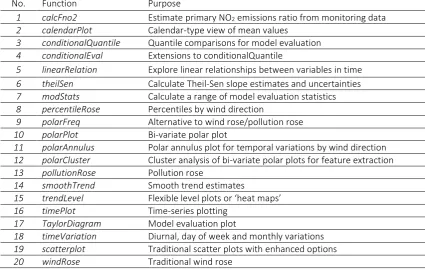
main analysis functions can be seen in Table 1.
Table 1 Main openair analysis functions
No. Function Purpose
1 calcFno2 Estimate primary NO2 emissions ratio from monitoring data
2 calendarPlot Calendar-type view of mean values
3 conditionalQuantile Quantile comparisons for model evaluation
4 conditionalEval Extensions to conditionalQuantile
5 linearRelation Explore linear relationships between variables in time
6 theilSen Calculate Theil-Sen slope estimates and uncertainties
7 modStats Calculate a range of model evaluation statistics
8 percentileRose Percentiles by wind direction
9 polarFreq Alternative to wind rose/pollution rose
10 polarPlot Bi-variate polar plot
11 polarAnnulus Polar annulus plot for temporal variations by wind direction
12 polarCluster Cluster analysis of bi-variate polar plots for feature extraction
13 pollutionRose Pollution rose
14 smoothTrend Smooth trend estimates
15 trendLevel Flexible level plots or ‘heat maps’
16 timePlot Time-series plotting
17 TaylorDiagram Model evaluation plot
18 timeVariation Diurnal, day of week and monthly variations
19 scatterplot Traditional scatter plots with enhanced options
For the purpose of this study, it discuses only six functions of openair model, which are
respectively theilSen for trend analysis, timeVariation for temporal variations, scatterPlot for
linear correlation analysis, timePlot for fluctuation analysis, windRose for wind rose creation,
and polarPlot for creating pollution rose based on the results from air quality studies in Jakarta
and Makkah using openair model application.
3.1
TheilSen Function
This function is useful in understanding concentration changes (trend) over a period of time and
for comparison with air quality standard. The result of this function is a slope value as the
percentage of trend changes and the value of the concentration changes in the unit per time
period. The increasing trend value is represented by the positive linear regression slope line
value while the decreasing trend value is represented by the negative slope of the linear
regression line.
The trend analysis of pollutant concentration using TheilSen Function is done based on
linear regression with Man Kendall method with 95% confidence interval and 5% significance
level (α). This confidence interval and level of significance can be adjusted to the limitations of
the study. The trend concentration change is also observed whether it tends to be significant or
not significant over the time period that occurs. In this case, an hypothesis is formulated in the
form of a significant trend change in pollutant concentration as an alternative hypothesis (Ha).
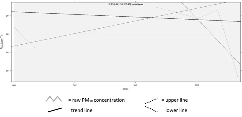
= raw PM10 concentration = upper line
= trend line = lower line
Figure 1 shows the application on Jakarta‘s PM10 data of 2016, which was a decrease
concentration change of PM10 concentration 5.73 µg/m3 per-year 2016. It was not significant
with p-value 0.85 (p-value> α). In this case, Jakarta needs to do more actions to reduce PM10.
3.2
Time Variation Function
Temporal variation of pollutant concentration can be described in the form of line graph to see
the fluctuation that happened in a certain time using timeVariation function. The result of this
function is an image consisting of four line graphs based on a specific time scale which are:
combination of hour-daily, hourly, daily, and monthly time. This function analyzes based on a
confidence interval 95%. The advantage of this function is able to plot more than one pollutant
in the same period of time.
By knowing the temporal variation of a pollutant over a period of time, the prediction can
be done in what time which the minimum or maximum concentration, in what day between
weekday or weekend the concentration will tend to be increasing or decreasing, in what month
the concentration will tend to be higher or low.
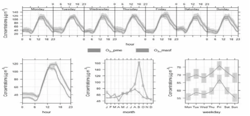
Figure 2 Time variation of O3 concentrations at the Presidency of Meteorology and Environment
(PME) and Masfalah monitoring sites in 2012 (Munir et al., 2015).
Figure 2 shows the temporal variation of O3 in two monitoring sites in Makkah during 2012.
The annual average of O3 concentration at the PME site (70.46 g/m3) was higher than the
Masfalah site (59.14 g/m3). The maximum O
Friday was the day with the highest O3 concentration. The month with the highest O3
concentration was September in PME and August in Masfalah (Munir et al., 2015).
3.3
ScatterPlot Function
Linear regression is used to see whether there is a correlation relationship between dependent
variable (pollutant concentration) and independent variable (meteorological factor). Linear
regression will yield the coefficient of determination (R2) which will interpret the result of
correlation/relationship. If indeed between two variables (meteorological factors and pollutant
concentration) have a relationship, the value of the relationship is analyzed whether it is
positive or negative.
Positive values will be identified with the slope of the upwardly sloped curve (the slope is
positive), while the negative value will be identified with the slope of the falling tendon (the
slope is negative). The direction of a positive relationship signifies a comparable relationship
such as the increased of the condition/value of the meteorological factor tends to be followed
by an increase in pollutant concentration. The direction of a negative relationship indicates a
reversed relationship that increases the condition/value of the meteorological factor tends to
be followed by a decrease in pollutant concentration.
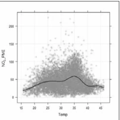
Figure 3 Scatter plots of NO2 and temperature at the Presidency of Meteorology and
A study by Habeebullah in 2015 found a negative correlation between NO2 concentrations
and temperature (Figure 3). The NO2 concentrations at PME monitoring site increase with
temperaturebut the concentrations of NO2 start decreasing after about 35C.
3.4
TimePlot Function
The result of timePlot function is a time series data with a pollutant data base over a period of
time. This function has advantages in terms of plotting several variables like more pollutant data
and meteorological data at once, but in the same period. This function will produce an up and
down line graph based on input data (without correction/interpolation). Fluctuations that
happen tend to describe the type of relationship that occurs whether positive or negative.
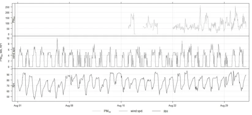
Figure 4 shows that no similar fluctuation is found between PM10, wind speed, and relative
humidity in the same period of August 2016 in Jakarta (Agustine, 2017). The type of relationship
between those three parameters is not conclusive. The relationships may be better explained
with the scatterPlot function discussed earlier.
Figure 4 Fluctuations of PM10 concentration, wind speed (wind spd.) and relative humidity (RH)
to ambient air of Jakarta in August 2016 (Agustine, 2017).
3.5
WindRose Function
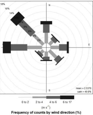
Wind rose illustrates how pollutant concentration, wind direction and speed vary over seasons.
Wind rose shows the dominant wind direction and the largest wind speed over a period of time.
The wind speed and direction indicate how far and where the pollutant is potentially dispersed
be identified by knowing the wind distribution. The scale of wind rose can be divided into
several wind directions such as eight wind directions for every 45. The wind is named based on
its origin, i.e. a north wind is a wind that originates in the north and blows south.
Figure 5 Windrose of Jakarta in 2016 (Agustine, 2017).
Figure 5 shows a wind rose analysis of Jakarta in 2016 studied by Agustine (2017). The
average wind speed was recorded at 2.5378 meters/second with calm condition 49.6%. Calm
condition means that wind speed is recorded at 0 meter/second. The dominant wind direction
was northwest (frequency by 13%) followed by west wind (frequency by 12.5%) with maximum
wind speed of 6 – 17 meters/second. Therefore, if there is a pollutant source in west and
northwestern area, it might be dominantly dispersed in east and southeastern area.
3.6
PolarPlot Function
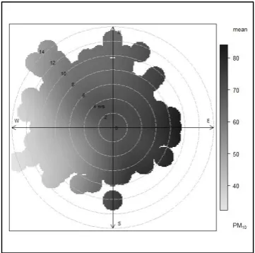
Pollution rose can identify the source and spatial distribution of air pollutants. The dominant
wind direction indicates the direction of emission dispersion from possible sources of pollutants
to the final polluted distribution area. Pollution rose as a development and variation of wind
rose is useful for considering spatial distribution of pollutant concentration dispersions based on
wind direction and speed to see the impact of air pollutant sources to the receptors. Some
pollutants are known to transport at various distance range, like PM10 transport from less than
Figure 6 Pollution rose of Jakarta in 2016 (Agustine, 2017).
Pollution rose of PM10 in Jakarta during 2016 can be seen in Figure 6. The analysis is based
on data from a monitoring station of BMKG in Central Jakarta. It identifies the PM10 pollutant
might be transported into area around southeast of Jakarta. The highest PM10 concentration are
recorded >80 μg/m3 in eastern and southeastern areas (Agustine, 2017). The analysis
represents PM10 pollutant dispersion all over Jakarta. However, the pollution rose result will be
better if the data come from several air quality monitoring stations.
4.
CONCLUSION
Openair model is a tool to analyze, interpret and understand air pollution data for better air
quality management. This model is based on statistical analyses definitely built for air quality
modeling such as linear regression, p-value's decision making and coefficient determination that
embedded to its various functions. Functions in openair model have their own utility purpose.
This study only examines six functions: theilSen for the analysis of pollution concentration
trends, timeVariation for the analysis of pollutant's temporal variations, scatterPlot for analysis
linear correlation between two variables, timePlot for analysis of pollutant and meteorological
factor's fluctuation, windRose for creating wind rose diagrams, and polarPlot for creating
pollution rose diagrams. Studies by Habeebullah (2015), Munir (2015), and Agustine (2017)
show that openair model is capable of performing various air quality data analyses for both
short time period (monthly) and long time period (yearly). Agustine (2017) shows the
application of openair model in Indonesia, exactly in Jakarta. The findings based on 2016 data
fluctuation between PM10 concentration, wind speed and relative humidity; the dominant wind
direction was northwest wind; the highest PM10 concentration >80 μg/m3 was dispersed in
eastern and southeast areas in Jakarta. The application of openair model in Indonesia is hoped
to increase more in the future with various air pollutants and lengthier period of time
monitoring.
5.
ACKNOWLEDGEMENT
The authors express gratitude to Meteorological, Climatological, and Geophysics Agency
(BMKG), Central Jakarta 10610
6.
REFERENCES
Carslaw, D. The Openair Manual Open-Source Tools for Analysing Air Pollution Data, King’s College, London, 2015.
Doucet, P., Sloep, P.B. Mathematical Modeling in the Life Sciences, King’s College, London,
1992.
Habeebullah, T. M. 2015. Characterising NO2, Its Temporal Variability and Association with
Meteorology: A Case Study in Makkah, Saudi Arabia. Journal of Environment Asia. 8(2): 37 – 44.
Agustine, I. Trend Analysis of Particulate Matter Less Than 10 Micron (PM10) to Ambient Air
Quality of Jakarta and Palembang. Thesis. Dept. Environmental Engineering, Universitas Trisakti. Jakarta, Indonesia, 2017.
Kurniawan, D. Regresi Linier (Linear Regression), R Development Core Team, R: A language and environment for statistical computing, R Foundation for Statistical Computing, Vienna, Austria, 2008.
Lelieveld, J., et al. 2015. The Contribution of Outdoor Air Pollution Sources to Premature Mortality on a Global Scale. Journal Nature. Vol. 525, page 367.
Munir, S. 2015. An Analysis into the Temporal Variations of Ground Level Ozone in the Arid
Climate of Makkah applying k-means Algorithms. Journal of Environment Asia. 8(1): 53 – 60.
Randall, T. Breathing Is Deadliest in These 15 Countries, Report of Bloomberg Business, 2015.
Tiwary, A., Colls, J. Air Pollution: Measurement, Modeling, and Mitigation, 3rd Edition, Routledge,