DESCRIBING THE HEIGHT GROWTH OF CORN USING
LOGISTIC AND GOMPERTZ MODEL
Wayan Surya Wardhani*) and Prawitra Kusumastuti
Faculty of Sciences, University of Brawijaya Jl. Veteran Malang 65145 East Java Indonesia
*) Corresponding author Phone:+62-341-554403 E-mail: [email protected]
Received: July 12, 2013/ Accepted: August 13, 2013
ABSTRACT
This paper is a critical study on corn (Zea mays) plant with a non linear approach, as it had slow growth rate at the initial stage of the cycle, followed by a rapid growth stage to a critical point then the height growth rate began to decline, reaching to a stability phase. The purpose of this research was to develop such a model to fit the height growth of corn (Zea mays) plant given microbial combination of Ochrobactrum sp.and Bacillus megatirium treatment; besides, to compare the plant absolute growth rate model between plant with microbial and non microbial treatment . A simple sigmoid model was preffered as it is easier to interpret the parameters biologically. The result showed that Logistic model fitted better in describing the height growth compared to Gompertz model, as it yielded coefficient of determination more than 99%. This model showed that the maximum height growth rate happened in about 40 day after planting. Based on the model, it showed that the absolute growth rate tended to be bell-shaped and right-skewed for Logistic and Gompertz, respectively.
Keywords : corn, Gompertz, height, Logistic, microbe
INTRODUCTION
Growth curve model is very useful for investigating growth problems in a short time especially in agricultural crops. Growth functions have been used to provide a mathematical summary about time data on the growth of an organism or part of an organism (Thornley and France, 2007). It allows us to test hypotheses and carry out virtual experiments concerning plant growth processes that can otherwise take
years in field conditions. The visualization of growth simulations allows us to see directly the outcome of a given model and provides us with an instructive tool useful for agronomists as well as for teaching. From a realistic point of view, such relationships among variables in agricultural sciences are non-linear in nature. And it was also said that the purpose of many agriculture researches was to increase the knowledge based component of agricultural production (Thornley and France, 2007). Then Paine et al., (2011) emphasized that plant growth was a fundamental ecological process and plant growth models are nowadays particularly important for describing biological processes with environmental conditions and provide the basis for more advanced researches in plant sciences. Besides, a Relative Growth Rate (RGR) is said to universally decrease as the size increases.
Corn is an important cereal crop after rice and it plays an important role for the people who live in rural areas. To fulfill the demand for corn to substitute rice, it is a must to have much knowledge about the growth process of the plant, such as collecting the height data of the plant. The plant height of corn plants at a certain growth stage may slightly vary depending upon planting date and growing conditions. In favorable conditions, generally, the plant height will be enhanced (Larson, 2013). There are many researches in corn growth that have been done : Williams II (2008) made an evaluation about the effect of planting date on height growth using analysis of variance, and to determine sweet corn height growth using logistic model. Estimating maize leaf area index and developing leaf area growth has been done by researchers (Karadavut et al., 2010); Yin et al., (2011) about improving a regression models between corn yield and corn plant height ; the
Accredited SK No.: 81/DIKTI/Kep/2011
result showed that there was a relationship between corn yield and plant height especially in multiple cropping system. Another research done was about a competition between pigweed redroot and the economic threshold in corn, where the result of the experiment showed that an increase of the corn density would (Vazin, 2012). Simple equation to show the plant growth pattern was needed; the growth in height at the beginning showed a slow growth, then it reached to a maximum, the growth model sh be derived ; calculating the first derivative allows us to find maximum growth rate and we can also draw a graph about the trend of that derivative of the model.
Statistical model is often insufficient to know in more details about the characteristic of the plant growth as it just tests whether there is a different effect of tratments to the plant variable. There were several studies about some non linear growth model in describing plant is a key indicator of plant growth and is linked to N nutrition during vegetative of corn development (Yin et al., 2011)
In relation with the growth model, statistic model would be applied to the data on corn plant height. The ability to estimate the mathematical model of plant height individually would benefit growers as they can plan the time when they must apply such an important treatment to have healthier plant in order to have good quality of corn yield and, thus, maximize their profits. Although it is difficult to forecast the corn to harvest, but knowing the height growth model of the plant is very helpful, as growers can determine the effective growth stage. Several methods of predicting and modeling crop yields have been used in the past with varying
success; but determining the individual growth model to determine the trend of growth rate at vegetative and generative phase and also the maximum growth rate has not done yet. Understanding what the trend of corn plant growth is the key to estimate the critical point of the growth stage.
The aim of the study was to estimate the trend of corn plant height growth data and chose the model whose parameter was easy to understand through Gompertz and Logistic model, and to see the trend of the absolute growth rate to determine the effective stage. The research result would be useful as an addition input of corn growth data base. Moreover, it is necessary to model the plant growth to realize when the critical period happens so that the plant breeders should apply a special treatment to the plant in order to increase the chances to a successful yield.
MATERIALS AND METHODS
Data Source
The height data used in this study were obtained from the experiment conducted at Physiology Laboratory of Biotechnology Departmentof PT BISI International in Kediri, East Java, from April to July 2011. The height data of Bisi B 816 corn variety was recorded every three days, started at 15 Days After Planting (DAP) to 81 DAP. The first group receiving the treatment of organic fertilizer of microbial combination of Ochrobactrum sp (as Nitrogen bounded) and Bacillus megatirium (as phos-phorous dissolved). Recommended Nitrogen fertilizer was applied to the second group, the control plant group. In this case, plant height could be used as an indicator of plant growth linked to Nitrogen nutrition during vegetative development of corn.
Statistical Analysis
Gompertz functions fitted the data, as simple sigmoid growth models, with four
parameters is where Y is
Logistic function is expressed as where Y is plant height, A is height potential,
is constant as time scale parameter, K is growth rate and t refers to time. This model is symmetric between its asymptotes; the lower asymptote is equal to 0 and the upper asymptote is Y=A; when t=0 we get Y=A/(1+
) as an initiation. The critical point indicated that the maximum growth rate occured when t = (ln
) / K and at that time the Y variable was about A/2.There were methods to obtain estimates of the unknown parameters of a non-linear regression model, as least square method was not easy work on, one of the method was Lavenberg-Marquardt method which is widely used for computing non linear least square.
The accuracy of models could be obtained based on Mean Square Error (MSE), coefficient of determination (R2) and Akaike Information Criterion (AIC) . Based on the analyses of the models, it could be verified that R2 values above 99%, indicate a good fitting model, with less MSE and smaller AIC (Kutner et al., 2004).
RESULTS AND DISCUSSION
Figure 1 demonstrates the scattered plot of corn height versus Days After Planting (DAP), measured from the field. There was a strong indication that sigmoid curve ought to be applied; the plant height grew rapidly then continued to form a plateau; Gompertz and Logistic growth model could be fitted to the data without difficulty by using nonlinear regression. Those models have three or four parameters that are biologically interpretable.
Figure 1. Scattered plot
It is clearly seen that there was a non linear or sigmoid trend in it. At about 60 DAP, the growth tended to be constant to infinite. So firstly we tried to fit with Gompertz model which the critical point, meaning that the growth rate reached the maximum at about 1/3 of the maximum growth. With Levenberg–Marquardt process, it was found that the Gompertz model
for height growth was
and ,respectively for the treated plant (plant given microbial treatment) and control plant (plant with no microbial treatment). From the assumption about normality using Kolmogorov-Smirnov test, it was found that p-value 0.85, greater than 0.05, meaning that the assumption about normality of the error was fulfilled; the homogeneity of the error variance was also fulfilled via J.Scroeter method test that yielded p-value of 0.82 which was more than 0.05 of significance. The R2 was 98.2 and 98.6 respectively, meaning that the variance of plant height was about 98% as explained by the model so it was an indication that the model was appropriate in describing the height growth of corn. The models yielded Mean Square Error (MSE) of 141.98 for treated plant and 111.28 for control plant ; AICGompertz statistic are 241.317 and 240.914 for treated and control plant respectively.
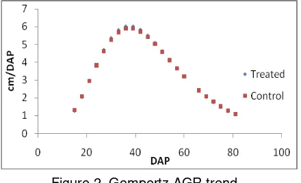
The next step was to find out the first derivative of the model showing how high (in cm) the plant grew per week; based on the first derivative, the trend of absolute growth rate is shown in Figure 2.
Figure 2. Gompertz AGR trend
equal to zero, it was found that the inflection point was at the coordinate of (37.39, 99.32) and (37.46, 98.53). It means that treated and control plant yielded the same result, where the maximum growth rate occurred at about 37 DAP and at that time the height of the treated and untreated plant was not significantly different.
Looking at the scattered plot, it could be possible to fit it with another sigmoid model such as Logistic. It was found that the model is :
with R2 of 99.2% and with R2 of 99.4% , for treated plant and control plant respectively, which means that more than 99% of the variation of height data is explained by the model, the rest of about 0.8% is explained by other strange variables. The MSE for these model were 64.98 and 43.88, and also the AICLogistic were 241.372 and 240.964, respectively.
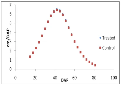
The first derivative of the model called absolute growth rate tended to be in bell shape. To determine when the maximum growth rate occurred, by the second derivative that equally to zero, the critical (inflection) point found to be (40.5,124.67) and (40.5,123.83) for treated and untreated plant respectively, which means that the maximum growth rate occurred at about 40-41 DAP and at that time the plant height was about 124 cm; furthermore, the analysis result shows that there was no significant difference at the plant height between treated and control plant. The following graph shows the trend of plant growth rate on Logistic model.
Figure 3. Logistic AGR trend
Comparing the coefficient of determination between two models, Logistic model was more
appropriate to be used to describe the height growth than Gompertz model as R2 Logistic was more than R2 Gompertz; besides, MSE from Logistic model was less than that of Gompertz and the AIC was more or less the same
As the critical time was at 40-41 DAP, it is important to the plant cultivator to look closer at the plant at that time, so that the growers could give a certain treatment to have better growth. This model is also suitable as database of corn plant growth.
CONCLUSION
Based on statistical approach Logistic model that fitted the data of corn growth better, as it gave higher coefficient of determination. The maximum growth rate occurred at 40-41 DAP and at that time the plant height was about 124 cm.
The mathematical model proposed herein seems to be adequate to study the growth of corn plant. However, other varieties, environment and growing conditions need to be taken into account. It is expected that there will be an accurate model to be applied in corn growth problem. As the corn plant goes through two stages as vegetative and generative stage, it would be better to study the plant growth in each plant stage whether there will be a different model of the two stages.
ACKNOWLEDGEMENTS
We wish to thank Bernadetha Mitakda for her careful approach and effective discussion in doing analytical methodology especially in growth modelling. Gratitude is also addressed to Loekito Adi Soehono as a senior researcher in experimental design.
REFERENCES
Amorim, L., A.B. Filho and B. Hau. 1993. Analysis of Progress of Sugarcane Smut on Different Cultivars Using Functions of Bouble Sigmoid Pattern. The American Phytopathological Society. Vol. 83 (9): 933-936
Hunt, R. 2003. Growth Analysis, Individual Plants. Growth and Development. people.exeter.ac.uk/rh203/EAPS_article. pdf . Access : April, 2012
Karadavut, U.,C.Palta., K.Kokten and A. Bakoglu. 2010. Comparative Study on Some Non-linear Growth Models for Describing Leaf Growth of Maize. International Journal of Agriculture & Biology. http://fspublishers.org. Access : October 2013.
Larson, E. 2013. How to Determine Growth Stages of Young Corn or Sorghum http://www.mississippi-crops.com/2013 /05/07/how-to-determine-growth-stages-of-young-corn-or-sorghum/. Access :No-vember, 2013.
Kutner,M.H., C.j. Nachtsheim and J. Neter. 2004. Applied Linear Statistical Models. Fifth Edition. McGraw-Hill. New York. Paine, C. E.T. , T. R. Marthews, D. R. Vogt,
D.Purves, M. Rees, A. Hector and L.A. Turnbull. 2011. How to fit Nonlinear Plant Growth Models and calculate Growth Rates : An Update for Ecologists. http://onlinelibrary.wiley.com/
doi/10.1111/j.2041210.2011.00155.x/ab stract.
Thornley,J.H.M. and J. France. 2007. Mathema-tical Model in Agriculture : quantitative methods for the plant, animal and ecological sciences. Cobi : London.books.google.co.id.
Vazin, F. 2012. The effects of pigweed redroot (Amaranthus retoflexus) weed compe-tition and its economic thresholds in corn (Zea mays). Planta daninha vol.30 (3) Viçosa July/Sept. 2012. http: //dx.doi.org /10.1590/S0100-835 82012000300003 Williams II, MM.2008. Sweet Corn Growth and
Yield Responses to planting Dates of the North Central United States. http://hort sci.ashspublications.org/content/43/6/17 75/full.pdf.