VEHICLE RECOGNITION IN AERIAL LIDAR POINT CLOUD BASED ON
DYNAMIC TIME WARPING
Tonggang Zhangab, George Vosselmanb, Sander J. Oude Elberinkb
a Faculty of Geosciences and Environmental Engineering, Southwest Jiaotong University, 610031 Chengdu, China - ([email protected]) b Faculty of Geo-Information Science and Earth Observation, University of Twente, 7500 AE Enschede, The Netherlands -
(George.vosselman, S.j.oudeelberink)@utwente.nl
Commission II, WG II/3
KEY WORDS: Vehicle recognition, Vehicle profile, Similarity measurement, Aerial Lidar, Dynamic time warping
ABSTRACT:
A two-step vehicle recognition method from an aerial Lidar point cloud is proposed in this paper. First, the Lidar point cloud is segmented using the region-growing algorithm with vehicle size limitation. Then the vehicle is recognized according to the profile shape based on dynamic time warping. The proposed method can detect vehicles parking under trees in an urban scene, and classifies the vehicles into different classes. The vehicle location, orientation, parking direction and size can also be determined. The experimental result based on a real urban Lidar point cloud shows that the proposed method can correctly recognize 95.1% of vehicles.
1. INTRODUCTION
Vehicle recognition from an aerial Lidar point cloud is a fundamental task for many Lidar applications, such as digital elevation model generation (Chen et al. 2017, Yang et al. 2016), urban parking management (Liu et al. 2016), traffic management and smart city modeling (Lafarge et al. 2012, Xiao et al. 2016).
To meet the requirements of these various applications and more potential further applications, the requirement of vehicle recognition can be divided into the two following aspects: 1) complete vehicle detection, which requires a high vehicle detection rate; 2) correct vehicle attributes, which include the vehicle class, location and size.
As to the first aspect, the current research cannot detect vehicles parked under or partially under trees (Börcs et al. 2015, Zhang et al. 2014), or detect vehicles parked too close to each other. However, the former is very common in the urban scene, especially with vehicles parked in side-streets. This is also the most important affecting factor. As to the second aspect, much research on vehicle classification has been performed based on the mobile Lidar point cloud (Xiao et al. 2016). Classifying a vehicle detected from ALS usually uses the spatial threshold, connection analysis (Rakusz et al. 2004), the profile shape buffer (Lovas et al. 2004), binary classification using object-based features (Yao et al. 2011) and the marked point process (Börcs et al. 2015). These methods focus on certain attributes of vehicles.
In this paper, a two-step method for vehicle extraction is proposed, including vehicle detection and recognition. It tries to collect as many vehicle segments as possible in the first step, and to remove the non-vehicle segments in the second step by vehicle recognition. In the first step, a vehicle size limitation is introduced to the procedure of non-ground points segmenting. The modification provides an opportunity to detect vehicles that are entirely or partially covered by trees. In the second step, the vehicle class is recognized by the similarity between the profile shape of the potential vehicle segment and a directed real vehicle profile based on dynamic time warping (Iglesias et al. 2013, Keogh et al. 2005). Other aspects, such as location and size, can also be estimated from the vehicle segment.
2. METHOD
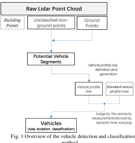
Supporting the ground point in the Lidar point cloud has been labelled. Vehicle detection and classification in this research contains two main steps. The first is to find as many potential vehicle segments as possible. The second is to identify whether a potential vehicle segment is a vehicle or not. By defining a vehicle profile, dynamic time warping is employed to measure the similarity between the profile derived from the potential vehicle segment and the standard vehicle profile. According to this index, the vehicle segment can be easily judged. The overall procedure of the proposed method is given in Fig. 1.
Fig. 1 Overview of the vehicle detection and classification method
2.1 Extracting potential vehicle segment with vehicle size limitation
The non-ground points are separated into different segments according to their spatial distribution. A segment is expected to either contain one vehicle or not contain a vehicle. During the separation, the size range of a real vehicle in terms of its width, length, and height direction is considered. The main steps of the potential vehicle segment extraction are given below.
Algorithm 1: Potential vehicle segment extraction
1. If point �� is not a ground point or building point (if the building classification is available),
a) If �� is the first point of the current segment, find the ground point in its neighboring range, and take the lowest ground point’s height as the ground height (��);
b) Create a segment using the region-growing algorithm taking �� as a seed point. During the growing, the next point �� should satisfy the following conditions:
0.3�<���− ��< max (��)
�(��,��) <�
where ��� is the height of point ��, �� is the height of the vehicle, �(��,��) is the horizontal distance between points (��,��), and � is a given threshold.
2. Estimate the width and length of the derived segment through its minimal boundary rectangle in the XOY plane. If both width and length satisfy the following condition, it will be judged as a potential vehicle segment
min (��) <����ℎ< max (��) min (��) <�����ℎ< max (��)
where ��and �� are the width and length of the vehicle,
respectively.
3. Add the potential vehicle segment into the segment list. 4. Repeat Steps 1 to 3, until all points are processed.
Step 1b) requires that the height of a point is no less than 0.3 m, to remove possible existing gross points around a vehicle, because the height of a vehicle’s top surface is not usually lower than 0.3 m.
Also, the tree points in the Lidar point cloud are mainly located on its top leaves and/or branches, which are usually higher than a vehicle. The maximal height in this condition is used to separate the tree points with the same plane position as a vehicle. This makes it possible to detect a vehicle entirely or partially parked under a tree.
To remove the segments which cannot possibly contain a vehicle, the limitation of the width and length of the segment is applied in Step 2.
To ensure that one segment only contains one vehicle, a threshold is set to separate vehicles according to the horizontal interval between two adjacent vehicles.
Using this method, each vehicle is expected in one segment. By setting slightly larger values for max (��), max (��) and
max (��), and slightly lower values for min (��) and max (��),
we can collect as many potential vehicle segments as possible for the next vehicle recognition step. Some of them may contain only a non-vehicle object.
2.2 Vehicle recognition using profile based on dynamic time warping
In this research, vehicle recognition refers to recognizing a vehicle by class, and not by type. A class level recognition is enough for vehicle modeling in the application of 3D urban modeling. That is to say, we only try to recognize a vehicle as a sedan, hatchback, SUV, or other class.
To recognize the vehicle, the profile of the potential vehicle segment is generated, and then compared with the real vehicle profile according to the similarity measurement derived by dynamic time warping (DTW).
2.2.1Vehicle profile generation: During acquisition of the Lidar point cloud, in most cases the laser point from the laser scanner mounted on the aircraft is not projected from a vertical direction, so the Lidar point cloud contains not only the points in its roof but also those on one or two sides. Of course, whether one or two sides are included is uncertain without additional data. And this depends upon the spatial position relationship between the vehicle and the laser scanner. Furthermore, for the top of the vehicle, its boundary is slightly uncertain owing to random sampling. Therefore, if the vehicle recognition is performed in 3D space, these uncertainties will create much trouble and difficulty.
To solve this problem, a vehicle profile is introduced. This is a curve of the middle part of the vehicle top side (Fig. 2). The curve reflects the vehicle shape, which provides enough information for further recognition. According to the position and character of the vehicle profile, it is obvious that the above two uncertainty factors are greatly reduced.
Fig. 2 The spatial relationship between the vehicle and profile
The detailed vehicle profile generation of one potential vehicle segment can be described as follows.
1. Determine the minimal boundary rectangle (MBR) in the XOY plane of one vehicle segment.
2. The central line of the profile is determined by the central point of the two shorter sides of the MBR. One is called the Begin point and the other is the End point (Fig. 3a). 3. Considering the points as randomly distributed, a buffer
along the central line is set. The width of the buffer depends upon the point density, and is 0.8 m in this paper.
4. Project all points {P(i)} in the buffer to the vertical plane through the central line along the horizontal direction. 5. Sort all projected points {P(i)} in ascending order of the
horizontal distance to the Begin point. The ordered array{P(i)} is called the vehicle profile (see Fig. 3b for an example), and it can also be considered as a directed curve.
{P(i)} =����(�),��(�)�� (1)
where ��(�) is the horizontal distance between the i-th projected points and the Begin point; ��(�) is the height difference between the i-th projected points and the ground height of the current segment.
(b) Vehicle profile. The horizontal axis is �� and the vertical axis is ��.
Fig. 3 Vehicle profile definition
2.2.2Vehicle profile recognition based on dynamic time warping: By introducing the vehicle profile, the question of vehicle recognition in 3-D space is simplified to curve recognition in 2-D space.
The profile provides information on the following three aspects: 1) the shape, 2) the height, 3) the length. The shape and height of the vehicle profiles of the same class look very similar, but differ greatly from other classes. But the length varies greatly with different types, even in the same class. For example, an economy sedan is usually shorter than a luxury one.
To achieve class-level vehicle recognition, the former two aspects should be considered, and third aspect should be neglected. Therefore, dynamic time warping (DTW) is employed to measure the similarity of two shapes with different lengths. If the profile is similar enough to the real profile of some class of vehicle, the vehicle can be recognized as the corresponding class.
In pattern recognition, dynamic time warping (DTW) is used for measuring the similarity between two time-series X, Y with different lengths. A well-known application is automatic speech recognition, to cope with different speaking speeds. Assume that �= [�1,�2,⋯,��] , �= [�1,�2,⋯,��], a �×� cost matrix � will be established with the distances between two points �� and �� , a warping path �=�1,�2,⋯,��
(max(�,�)≤ � ≤ �+� −1) is formed by a set of matrix components, subject to the following boundary condition �1=
�(1,1), ��=�(�,�), monotonicity and a step size condition of ��. The minimized warping cost �is considered as the
similarity measurement (Iglesias et al. 2013, Keogh et al. 2005).
�=����∑��=1�� (2)
If two time-series are of the same shapes, � equals 0, even with different lengths; it will be greater than 0 when they are of different shapes. The more similar, the lower the value of �, and vice versa.
The vehicle profile {P(i)} is a point series sorted in ascending order of its distance (see Eq. (1)). {P(i)} can be regarded as a pseudo time-series, taking the distance as the “time”, and the height as the signal. Then dynamic time warping (DTW) can be employed to measure the similarity to a real vehicle profile.
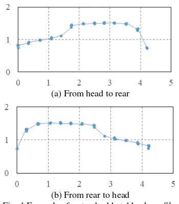
Because dynamic time warping (DTW) aligns two time-series in time order, two identical time-series in reverse order will be recognized as different. Considering that it is difficult to judge the vehicle’s direction in a Lidar point cloud, two directed profiles are prepared for one type of vehicle in reverse order. See Fig. 4 for an example. According to this characteristic, the Begin point of the vehicle profile corresponding to the vehicle’s head or tail can be determined. That is, additional information, namely the parking direction, can also be obtained.
(a) From head to rear
(b) From rear to head
Fig. 4 Example of a standard hatchback profile. (The horizontal axis is �� and the vertical axis is ��.)
Algorithm 2: Vehicle recognition using dynamic time warping (DTW)
1. Create vehicle profile set {��������_��ℎ����_�������(�)} (0 <� ≤2�) for different vehicle classifications. n is the number of vehicle classifications considered.
2. Derive the vehicle profile {�������_��ℎ����_�������(�)} of the i-th potential vehicle segment.
3. Calculate the similarity measurement D(�,�) between
{�������_��ℎ����_�������(�)} and each vehicle profile in
{��������_��ℎ����_�������(�)}
∃� ∈[0,�], D(�,�) =��� (3)
4. If D(�,�) is no larger than the threshold, the i-th potential vehicle segment is recognized as a vehicle, and its class is the same as that corresponding to the m-th standard vehicle profile; if D(�,�) is larger than the threshold, it is recognized as a non-vehicle object.
5. Repeat Steps 2 to 4, until all derived vehicle profiles are recognized.
3. EXPERIMENT
3.1 Experimental dataset
3.1.1Lidar point cloud: The test area is a common block located in Enschede, the Netherlands. The Lidar point cloud is extract from the AHN2 dataset, which was obtained in 2008 with a point density of 20–30 pts/m2 (Fig. 5). The average distance between two arbitrary neighboring points is about 0.2 to 0.3 m. The area is about 200m by 120m.
Fig. 5 Lidar point cloud of test area
A manual visual inspection will be employed to check the result of our method.
3.1.2 Standard vehicle profiles: Considering that most vehicles are small- or middle-sized in the urban area, five vehicle classes are considered: sedan, hatchback, sedan wagon, compact and middle-sized van, and SUV (Table 1).
Buses and coaches are not considered because they usually park in special parking lots. Trucks are also not considered as they are rarer in urban areas.
Table 1 Vehicle classes and their profiles Vehicle
class Vehicle profile Picture
Sedan
Hatchback
Sedan Wagon
Compact and
middle-sized van
SUV
These five profiles (Fig. 6) and five corresponding reverse order profiles are used in the experiments.
Fig. 6 Standard vehicle profiles
3.2 Potential vehicle segment detection
The potential vehicle segments are first extracted. This step is very important. A vehicle not detected in this step will be missed in the result. The parameters for the Lidar segment are determined by investigating the sizes of different vehicles, and the range of vehicle widths and lengths is set as
��∈(1.4�, 1.9�),��∈(2.7�, 6.5�)
and vehicle heights ��< 3.1�.
The threshold (�) for separating segments is set to 0.5 m. The detected vehicle segments are shown in Fig. 7.
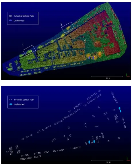
Fig. 7 The detected potential vehicle segments
From Fig. 7, 92 potential vehicle segments are obtained, denoted by blank rectangles, where 13 vehicles are entirely or partially parked under trees. 14 of the segments are non-vehicles, and 4 vehicles are not detected (denoted by solid ellipses).
Fig. 8 Vehicles parked under a tree
Vehicle #1 is partially covered by a tree, and vehicles #2 and #3 are entirely covered by a tree. They are all detected correctly. This is because the height range is set to 0.3–3.1m (denoted by the solid white lines in Fig. 8), so most tree points are excluded during the potential vehicle segmentation.
3.3 Vehicle recognition
Therefore, the profile of each vehicle segment is produced first, and is then recognized using dynamic time warping (DTW). The threshold of similarity measurement is set to 7. The vehicle recognition results are given in Fig. 9.
Fig. 9 The derived vehicle classification
After manually checking the results, all the vehicles are identified correctly, and the 13 non-vehicle segments are also identified correctly. No non-vehicle segments are recognized as vehicles.
3.4 Vehicle detection accuracy
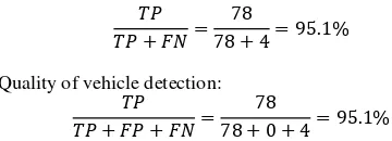
To quantitatively evaluate the accuracy of the proposed method, three indexes, correctness, completeness and accuracy, are used. Correctness is��/(��+��), completeness is ��/(�� +
��)and quality is ��/(��+��+��); where TP is the sum of true positives, FP is the sum of false positives and FN is the sum of false negatives (Powers 2011, Tuermer et al. 2013).
The statistics of vehicle recognition are listed in Table 2.
Table 2 The vehicle detection count Vehicle Non-vehicle Detected vehicle TP=78 FP=0 Detected non-vehicle FN=4 TN=14
The 4 undetected vehicles are also counted in Table 2. Correctness of vehicle detection: proposed method is 95.1% overall.
4. CONCLUSION
The vehicle recognition method first separates the Lidar point cloud into segments with the vehicles’ size limits. Then the segment can be further recognized by the similarity measurement between its profile and standard vehicle profiles. Dynamic time warping (DTW) is employed to estimate the similarity of the profiles.
The similarity measurement can be calculated by dynamic time warping (DTW). The experimental results show that the accuracy of the proposed method is 95.1%.
During the Lidar point cloud segmentation, the vehicle’s size, i.e., width, length, and height, is considered. This makes it possible to extract a vehicle that is covered or partially covered by trees, which is very common in urban areas.
Vehicles in the same class have similar shapes, but vary in length according to the different types. The similarity measurement derived by DTW is less affected by the vehicle length, and it provides a good solution for identifying the class of vehicle.
REFERENCES
Börcs A. and Benedek C., 2015. Extraction of vehicle groups in airborne Lidar point clouds with two-level point processes. IEEE Transactions on Geoscience and Remote Sensing, 53(3), pp. 1475-1489.
Chen Z., Gao B. and Devereux B., 2017. State-of-the-art: DTM generation using airborne lidar data. Sensors, 17(1), pp. 150. Iglesias F. and Kastner W., 2013. Analysis of similarity
measures in times series clustering for the discovery of building energy patterns. Energies, 6(2), pp. 579-597. Keogh E. and Ratanamahatana C. A., 2005. Exact indexing of
dynamic time warping. Knowledge and Information Systems, 7(3), pp. 358–386.
Lafarge F. and Mallet C., 2012. Creating large-scale city models from 3D-point clouds: A robust approach with hybrid representation. International Journal of Computer Vision, 99(1), pp. 69-85.
Liu Y., Monteiro S. T. and Saber E., 2016. Vehicle detection from aerial color imagery and airborne lidar data. In: 2016 IEEE International Geoscience and Remote Sensing Symposium (IGARSS), Prague, Czech, pp. 1384-1387. Lovas T., Toth C. K. and Barsi A., 2004. Model-based vehicle
detection from lidar data. In: The International Archives of the Photogrammetry, Remote Sensing and Spatial Information Sciences Istanbul, Turkey,B4, pp. 134-138. Powers D. M. W., 2011. Evaluation: From precision, recall and
f-measure to roc, informedness, markedness and correlation. Journal of Machine Learning Technologies, 2(1), pp. 37-63. Rakusz Á., Lovas T. and Barsi Á., 2004. Lidar-based vehicle
segmentation. In: The International Archives of the Photogrammetry, Remote Sensing and Spatial Information Sciences Istanbul, Turkey, pp. 156–159.
and disparity maps. IEEE Journal of Selected Topics in Applied Earth Observations and Remote Sensing, 6(6), pp. 2327-2337.
Xiao W., Vallet B., Schindler K. and Paparoditis N., 2016. Street-side vehicle detection, classification and change detection using mobile laser scanning data. ISPRS Journal of Photogrammetry and Remote Sensing, 114(4), pp. 166-178.
Yang B., Huang R., Dong Z., Zang Y. and Li J., 2016. Two-step adaptive extraction method for ground points and breaklines from lidar point clouds. ISPRS Journal of Photogrammetry and Remote Sensing, 119, pp. 373-389.
Yao W., Hinz S. and Stilla U., 2011. Extraction and motion estimation of vehicles in single-pass airborne lidar data towards urban traffic analysis. ISPRS Journal of Photogrammetry and Remote Sensing, 66(3), pp. 260-271. Zhang J., Duan M., Yan Q. and Lin X., 2014. Automatic vehicle