Spatial and temporal dynamics of vegetation in the
San Pedro River basin area
J. Qi
a,∗, R.C. Marsett
b, M.S. Moran
b, D.C. Goodrich
b, P. Heilman
b,
Y.H. Kerr
c, G. Dedieu
c, A. Chehbouni
d, X.X. Zhang
eaDepartment of Geography, Michigan State University, 315 Natural Science Building,
East Lansing, MI 48824-1115, USA
bUSDA–Agricultural Research Service, Tucson, AZ, USA cCESBIO, Toulouse, France
dIRD/IMADES, Hermosillo, Mexico
eCenter for Space Science, Applied Research, Chinese Academy of Science, Beijing, China
Abstract
Changes in climate and land management practices in the San Pedro River basin have altered the vegetation patterns and dynamics. Therefore, there is a need to map the spatial and temporal distribution of the vegetation community in order to understand how climate and human activities affect the ecosystem in the arid and semi-arid region. Remote sensing provides a means to derive vegetation properties such as fractional green vegetation cover (fc) and green leaf area index
(GLAI). However, to map such vegetation properties using multitemporal remote sensing imagery requires ancillary data for atmospheric corrections that are often not available. In this study, we developed a new approach to circumvent atmospheric effects in deriving spatial and temporal distributions of fcand GLAI. The proposed approach employed a concept, analogous
to the pseudoinvariant object method that uses objects void of vegetation as a baseline to adjust multitemporal images. Imagery acquired with Landsat TM, SPOT 4 VEGETATION, and aircraft based sensors was used in this study to map the spatial and temporal distribution of fractional green vegetation cover and GLAI of the San Pedro River riparian corridor and southwest United States. The results suggest that remote sensing imagery can provide a reasonable estimate of vegetation dynamics using multitemporal remote sensing imagery without atmospheric corrections. © 2000 Elsevier Science B.V. All rights reserved.
Keywords: Remote sensing; Spatial and temporal dynamics; San Pedro River basin; Fractional cover; Green leaf area index
1. Introduction
Climate change and increasing human activities have resulted in a substantial change in the vegetation type and distribution in the southwest United States. Chihuahuan desert shrubs and mesquite trees increas-ingly have become dominant and replaced native
∗Corresponding author. Tel.:+1-517-353-8736;
fax:+1-517-432-1671.
E-mail addresses: [email protected], [email protected] (J. Qi).
grasses over large areas (Kepner et al., 1998; Watts et al., 1998). The change in vegetation pattern has a feedback influence on the local and regional climate by reducing evaporative water losses from surface to atmosphere. Therefore, the spatial and temporal distributions of vegetation characteristics is important in understanding how climate and human activities affect the ecosystem in the semi-arid environment.
Estimation of vegetation properties with remotely sensed imagery has been quite successful. How-ever, when applied to satellite imagery, tremendous
processing efforts related to atmospheric and bidirec-tional corrections are needed. Although procedures to correct these effects are available, ancillary data about atmospheric conditions and bidirectional prop-erties of the surface types are limited in both space and time. This has prevented satellite data from being used to quantify vegetation dynamics for practical ap-plications. A common practical technique to correct atmospheric effect is dark-object subtraction (Chavez, 1988; Caselles and Garcia, 1989), which subtracts the minimum pixel values of a dark object found in a scene with an assumption that no energy is reflected from that dark object. However, in many cases, it is impossible to find a dark object within a scene that is large enough to occupy more than one single pixel, especially when coarse spatial resolution satellites are used. An alternative is to use pseudo invariant objects (PIOs) within a scene to convert digital numbers to radiance or reflectance values (Schott et al., 1988; Moran et al., 1996, 1997). PIOs are those objects whose reflectances are known and remain approxi-mately constant throughout time and therefore can be used to “calibrate” multitemporal images.
Reflectance properties of most PIOs, however, vary with many factors such as surface conditions. When bare soil fields are used as PIOs, e.g., their reflectances vary with soil moisture content and surface rough-ness, which changes throughout the season because of the impact of rainfall events. Use of either a dark object or a PIO for atmospheric corrections will not correct for bidirectional effects. When an image is ac-quired at an oblique view, the reflectance properties of most objects including PIOs may vary substantially. Therefore, oblique viewing will introduce a constant bias when PIOs are used for atmospheric corrections. Noise associated with atmospheric and bidirectional effects will be magnified when calculating derivative products such as vegetation cover and biomass, es-pecially over sparsely vegetated surfaces. Thus, it is critical that methods be developed to circumvent at-mospheric and bidirectional effects. The objective of this study is to develop an alternative technique to de-rive remote sensing products such as fractional green vegetation cover (fc) and leaf area index (LAI) that are
less sensitive to atmospheric effect. Although viewing angles may introduce errors in estimated fc and LAI,
no attempt was made to correct bidirectional effects in this study.
2. Methodology
By definition, a PIO is an object whose reflectance properties are invariant throughout time. Examples of such objects are bare soil fields, airstrips, and highways. Therefore, multitemporal remote sensing images can be converted to surface reflectances by us-ing a linear relationship between raw digital numbers on the image and the known reflectances of the PIOs found within the scene. The key assumption is that the object is invariant in terms of surface reflectance. This assumption, however, is not valid for most nat-ural land surfaces because their reflectance properties are known to vary with many external factors such as surface conditions and sensor’s viewing angles. Therefore, the fundamental assumption of invariance in reflectance fails in most cases, resulting in uncer-tainties in surface reflectance and its derived products. There are other physical properties besides reflec-tances that are indeed invariant with time and surface conditions. Such physical properties include the pres-ence of vegetation or green biomass. For example, a bare soil field, which is often used as a PIO, changes in surface reflectance with surface moisture condition, roughness, and sensor/sun-viewing angles. However, the fractional green vegetation cover (fc) or green leaf
area index (GLAI) does not vary with these factors. Therefore, the bare soil field is variant in surface re-flectances but invariant in green vegetation cover or green biomass, allowing one to use this truly invari-ant property to calibrate the green cover product rather than to calibrate reflectance.
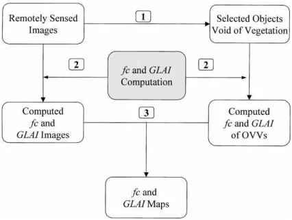
Fig. 1. Flow chart of the approach to compute green vegetation cover (fc) and GLAI using OVVs.
of OVVs may not be zero and need to be adjusted. The second step is to compute this non-zero adjust-ment factor in terms of fractional cover and GLAI (algorithms for computing these two variables are de-scribed below). The third and final step is to compute the fc and GLAI spatial distribution by subtracting
the adjustment factor from the entire image.
In this study, we focused on the derivation of tem-poral dynamics of vegetation in the San Pedro River basin where the semi-arid land-surface-atmosphere (SALSA) program is currently focusing its effort (Goodrich et al., 2000). In particular, we used the proposed adjustment approach to derive spatial and temporal distributions of the fractional green vegeta-tion cover (fc) and GLAI of the study area. The
se-lected OVVs in this study included the Wilcox playa, Arizona for all TM images and White Sands, New Mexico for the VEGETATION images. These OVVs can also be used as PIOs. The fc and GLAI values
of the Wilcox playa and White Sands were computed and subtracted from the entire fc and GLAI images.
The fc and GLAI values of these OVVs provided
baselines for each image to allow an automatic adjust-ment of the fc and GLAI values from multitemporal
remote sensing imagery.
2.1. Green vegetation cover estimate
Fractional green vegetation cover (fc) in arid and
semi-arid regions is an important variable in
hydrolog-ical and ecologhydrolog-ical modeling studies. Their temporal dynamics and spatial distributions are often needed in global circulation models (GCMs) in order to compute the energy or water fluxes. Estimation of fractional green vegetation cover, fc, from remotely sensed data
is often associated with computation of spectral veg-etation indices and their empirical relationships with fractional green vegetation cover. In this study, we used a linear mixing model to relate fc with spectral
vegetation indices.
Assume that a pixel signal consists of the contri-bution from two components: soil and vegetation. Let the fractional green vegetation cover be fcand,
there-fore, the fractional soil cover would be 1−fc. The
resulting signal, S, as observed by a remote sensor can be expressed as
S=fcSv+(1−fc)Ss (1)
where Svis the signal contribution from the green
veg-etation component and Ss from the soil component.
For pixels consisting of more than two components, Eq. (1) needs to be modified. This analysis assumed that a pixel consisted of only vegetation and soils. Eq. (1) can be applied to remotely sensed data in the reflectance domain (Maas, 1998) and in the spectral vegetation index domain (Zeng et al., 2000). When ap-plied with a spectral vegetation index such as the nor-malized difference vegetation index (NDVI), Eq. (1) may be approximated by
NDVI=fc×NDVIveg+(1−fc)NDVIsoil (2)
which can be re-written as
fc=
NDVI−NDVIsoil
NDVIveg−NDVIsoil
(3)
where NDVIsoil is the NDVI value of an area of bare
soil or OVV, and NDVIvegis the NDVI value of a pure
vegetation pixel.
Although many vegetation indices are available, we selected NDVI because of its traditional use in deriv-ing vegetation variables. The NDVIsoil values should
be constant throughout time and close to zero in theory for most type of bare soil surfaces. However, due to at-mospheric effect, and changes in surface moisture con-ditions, NDVIsoil values vary substantially with time.
for the entire image may not be valid unless the area of interest consists of uniform soil types. For this rea-son, we selected surfaces near the center of an image to minimize errors associated with variations in NDVI values of OVVs. To use the proposed adjustment ap-proach, it is not necessary to know the exact values of NDVIsoilbecause this value will be computed from
each image. The NDVIsoil values from each image
were used to compute the associated fc and GLAI
adjustment factors.
As previously stated, the spatial variation of bare soil surfaces may also be related to the sensor’s observation angles. Therefore, depending on the sun-viewing geometry of each pixel, the selected NDVIsoil may be different and thus result in
uncer-tainties in fc and GLAI estimation. To minimize the
bidirectional effect, it is suggested to avoid large view angle data when nadir-looking images are available. In this study, the nadir-viewing TM images were used in the analysis. The proposed adjustment approach was designed to circumvent primarily the atmospheric effect, aiming at analyzing vegetation dynamics from multitemporal images. Uncertainties were expected when using images acquired with large viewing angle sensors.
The value for NDVIveg represents the maximum
value of a fully vegetated pixel. Because of the tem-porally dynamic nature of green vegetation cover, this value needs to be empirically determined. In selecting such a value, we examined all images and selected an image acquired during the peak-growing season within the area of interest. The NDVIveg was determined in
this study to be 0.8 from high spatial resolution data. During the selection process, surfaces of known to be 100% green cover were identified and the correspond-ing NDVI values were computed from multitempo-ral images, and then the highest value (0.8) was used for all image. This empirically determined value may also vary with atmospheric conditions (Kaufman and Tanre, 1992; Qi et al., 1994), which may cause some errors in the fractional cover computation in Eq. (3).
Because the NDVI is a ratio vegetation index, it can be directly computed with digital numbers, or with top of atmosphere radiance or reflectance, or surface reflectance. In this analysis, NDVIveg of 0.8 was
de-termined using surface reflectances derived from TM images. When used with radiance, or digital num-bers, or top-of-atmosphere reflectance or radiance, the
NDVIveg may be different. However, once the data
type (radiance, raw digital numbers, or top-of-atmos-phere reflectance or radiance) is determined, the NDVIveg should be constant.
2.2. GLAI estimate
Another important vegetation characteristic is the GLAI. Unlike the fractional green vegetation cover, which is a two-dimensional horizontal variable, the GLAI is a variable describing the density of green vegetation. It is defined here as the total single-side area of green leaves per unit ground area. Therefore, its values can theoretically range from 0 to∞, whereas fcranges from 0 to 1.
Approaches to derive GLAI exist using either em-pirical relationships with spectral vegetation indices or model inversion techniques. For arid and semi-arid regions such as the San Pedro River basin, we adapted the approach by Qi et al. (2000), which was de-rived using a combination of modeling and empirical approaches
GLAI=aNDVI3+bNDVI2+cNDVI+d (4) where a, b, c, and d are empirical coefficients and were found to bea =18.99,b= −15.24,c=6.124, and
d= −0.352 for arid and semi-arid regions. The GLAI values derived from these coefficients were validated using TM imagery data over a desert grassland, and therefore, the use of them over a large area of diverse vegetation remains to be further validated. Since the TM imagery used in this study covered the same geo-graphic areas, it is expected that uncertainty in GLAI estimation from these coefficients would not be signif-icantly different from the original study. Furthermore, if adjusted NDVI was used in Eq. (4), the coefficient d should be adjusted to zero to ensure that the GLAI values of OVV were zeros for all seasonal images.
3. Data description
3.1. Remote sensing data
Table 1
Remote sensing images acquired in 1992, 1997, and 1998 over the study area in the southwest United States on different dates and DOY
Airborne TMS Landsat TM SPOT 4 VEGETATION
Date DOY Date DOY
16 February 1997 46 Daily from 30 April to 30 December 1998
20 March 1997 79
21 April 1997 111
24 April 1992 114
8 June 1997 159
11 June 1992 162
12 August 1997 224 27 June 1992 178
13 July 1992 194
Spatial resolution: 3 m Spatial resolution: 30 m Spatial resolution: 1000 m
registered to UTM coordinates. A total of 15 Land-sat TM images were acquired in 1992 and 1997 over the San Pedro basin area (Table 1). Thematic mapper simulator (TMS) was deployed on an aircraft during the SALSA intensive field campaign in August 1997 (Goodrich et al., 2000) to acquire images at a 3 m spa-tial resolution. Daily SPOT 4 VEGETATION images were acquired over this study area at a spatial resolu-tion of 1000 m. Therefore, the remotely sensed images had a range of spatial resolution from 3 m to 1 km. In addition to these satellite- and aircraft-based remote sensing data, surface reflectances were also measured at the Audubon ranch near Elgin, AZ, in 1998, us-ing an MMR radiometer in the same spectral bands as Landsat TM sensor.
3.2. Vegetation data
Ground vegetation properties were recorded in 1992, 1997 and 1998 using both destructive sampling technique and Li-Cor’s LAI-2000 instrument. Vege-tation samples were collected at three study sites. The first site was located in the center of Walnut Gulch Experimental Watershed and the site was dominated by tobosa grasses (Hilaria mutica) with some desert shrubs. The second site was near the Lewis Springs within the San Pedro River basin and the dominant grass was sacaton (Sporobolus wrightii). The third site
was at the Audubon research ranch near Elgin, AZ, and the dominant vegetation types were native upland grasses, Lehmann’s lovegrass, and sacaton grasses.
Both destructive and non-destructive methods were used to measure the GLAI. For the destructive method, vegetation samples were collected in the field and brought back to the lab and separated into green vege-tation, senescent vegevege-tation, and litter. The single side leaf areas were measured by passing them through an LAI-3000 area meter for each component and GLAI was then computed. For the non-destructive method, LAI-2000 instrument was used to measure total LAI, and the lab-based ratio of green to total leaf areas was used to compute the GLAI. Measurements of the to-tal fractional vegetation cover were made by visual estimate on site during each field visit. Detailed de-scriptions of this data set can be found in Moran et al. (1998). The ground in situ measurements were then used in this study to examine the effectiveness of the proposed approach.
4. Results
4.1. Spatial dynamics of green vegetation
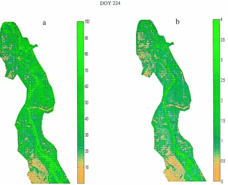
Fig. 2. Spatial distribution of green vegetation cover (a) and GLAI (b) derived from TMS images (3 m resolution) over a portion of the San Pedro basin near the Lewis Springs, AZ.
resolution TMS data (Fig. 2). The spatial extent cov-ered the riparian corridor of the San Pedro River from Hereford to Fairbanks (see Fig. 2 in Goodrich et al., 2000). Dense green vegetation cover was distributed along the river where the cottonwood–willow riparian forest gallery was located. Away from the riverbanks toward the upland areas, the green vegetation cover diminished. There was also a vegetation cover gradi-ent from Fairbanks to Hereford or from north to south of the study area. This gradient was most likely due to water availability from the river and weather pattern variation due to elevation changes. Along the river were cottonwood and willow trees, which require
vegetation cover of the sacaton was thus less than the cottonwood–willow community and mesquite trees.
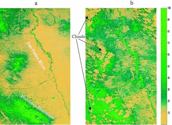
4.2. Temporal dynamics
To examine the temporal dynamics of vegetation in the San Pedro River basin, a portion of the basin was extracted from two Landsat TM images acquired on 21 April (DOY 111) in the dry season and on 12 September (DOY 255) in the wet season of 1997. The spatial distribution of green vegetation cover (Fig. 3) and GLAI (Fig. 4) of the two seasons covered a portion of the San Pedro River basin. Note the scale difference between Figs. 3 and 4. The Huachuca mountains are located at the lower left corner of the images. The spotty areas with yellow color on the left-hand side of Figs. 3b and 4b were clouds. The dry season was characterized with little green vegetation while the wet season, due to increased precipitation, produced more green vegetation cover. In the dry sea-son, only the river and mountainous areas had green vegetation. In the wet season, cottonwood, willows and mesquite trees were green. The sacaton, in spite
Fig. 3. Green vegetation cover maps derived from TM imagery of: (a) 21 April 1997, DOY 111; (b) 12 September 1997, DOY 255.
of possible new growth underneath the canopy, did not appear green. Due to increased precipitation dur-ing the monsoon season, the wet season (Figs. 3b and 4b) had more green vegetation than the dry season (Figs. 3a and 4a).
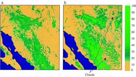
4.3. Large scale vegetation cover and GLAI
Fig. 4. GLAI maps derived from TM imagery of: (a) 21 April 1997, DOY 111; 12 September 1997, DOY 255.
Fig. 6. GLAI maps derived from SPOT 4 VEGETATION imagery of: (a) 21 April 1998, DOY 111; (b) 12 September 1998, DOY 255.
little detailed structures (Figs. 5 and 6) in comparison with those derived from TM images (Figs. 3 and 4). Clearly, the San Pedro River can be seen with TM derived maps (Figs. 3 and 4), but can barely be seen on VEGETATION derived maps in Figs. 5 and 6.
5. Validation
Because of only limited ground-based data avail-able for this study, it was difficult to fully validate the proposed adjustment approach. However, inter-comparison of results from different data sets was made in three ways to verify the adjustment approach: (1) intercomparison across atmospheric corrections, (2) intercomparison across spatial scales, and (3) comparison against ground in situ data.
5.1. Across-atmosphere comparison
For this analysis, we selected 1992 TM images because of availability of ancillary data for atmo-spheric corrections. A window of 9×9 pixels, a size of approximately 270×270 m2area near Tombstone
within the Walnut Gulch Experimental Watershed, was extracted from all 1992 TM images. The mean values of reflectance at the surface (with atmospheric correction) and at the top of atmosphere (without atmospheric correction) were used to compute multi-temporal NDVI values. These values were then used in Eqs. (3) and (4) to compute temporal dynamics of fcand GLAI values without any adjustment. The data
Fig. 7. Comparison of fractional cover values derived with data before and after atmospheric correction, and with the proposed approach using the data without atmospheric correction.
approach could reduce the atmosphere-induced noise in the temporal vegetation dynamics estimated from TM images even though no atmospheric correction was made.
5.2. Across-scale comparison
The remotely sensed data used in this analysis had a range of spatial scales from 3 to 1000 m (Table 1). To compare results across spatial resolutions, a common area (5×1 km2) found in both TMS (3 m) and TM (30 m) images was extracted and the statistical means were computed. This could not be done with VEGE-TATION images because the TMS coverage was not enough to cover even a single pixel of the VEGETA-TION data. To compare spatial scales between TM and VEGETATION, a separate common area (5×5 km2) was extracted and statistical means were used for intercomparison. Due to limited TMS data, we could only compare TMS with TM for the wet season, while comparison between TM and VEGETATION was made for both dry and wet season. The results were plotted in Fig. 8. Although the spatial scales were different, the mean values of the fractional green cover estimated at three spatial scales agreed well. Because the TMS image was acquired over the inten-sive study site at the Lewis Springs site of SALSA
program and had a spatial resolution of 3 m, we felt quite confident about the fcestimate with this image.
Therefore, the estimated fc from the fine resolution
TMS image could be used to assess the accuracy of fc estimates by the coarser resolution TM and
VEG-ETATION images. The good agreement among all three scales (Fig. 8) suggest that the estimated fcwith
TM and VEGETATION images had approximately the same accuracy of that estimated by TMS image.
5.3. Comparison with in situ measurements
In this analysis, we selected 1997 TM images be-cause of availability of ground in situ measurements of fractional cover and GLAI from the SALSA program and other research projects at the three study sites de-scribed previously. The estimated fcand GLAI values
for this analysis were all derived from 1997 TM im-ages without atmospheric corrections to demonstrate the effectiveness of the adjustment approach for reduc-ing atmospheric perturbation. Because of rigid Land-sat Land-satellite overpass schedules over the study sites, the ground in situ measurements were not always co-incident with the satellite overpass dates.
Fig. 8. Comparison of fractional green cover estimated using the proposed approach at different spatial scales: 3 m (TMS), 30 m (TM) and 1000 m (VEGETATION).
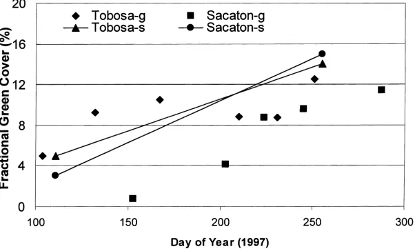
presented in Fig. 9. The in situ fc values agreed
rea-sonably well with those derived from TM images. The seasonal trends of the estimated fc were reasonably
well in agreement with those observed on the ground. In spite of the fact that there was a good agreement between estimated fc values and in situ
measure-ments, no conclusive statements could be made, due to limited number of data available for this analysis.
Fig. 9. Comparison of ground-based green vegetation covers (as indicated with a suffix g) with those estimated using satellite imagery (as indicated with suffix s) for tobosa and sacaton grasses using the proposed approach.
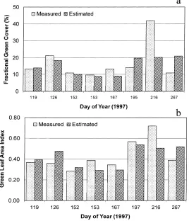
For the Audubon study site, both fractional green cover (fc) and GLAI values were derived using
ground-based reflectance measurements with the ad-justment approach. The computed fcand GLAI values
Fig. 10. Comparison of in situ fractional green cover (a) and GLAI (b) measurement with those derived using the proposed approach and ground-based reflectance measurements at Audubon site, where native grasses and Lehmann lovegrass were dominant species.
vegetation cover, fc, was underestimated by
approx-imately 50%. This unexpected discrepancy on this date could be due to several factors. One was the het-erogeneous nature of the study areas. Since ground sampling was made within several 2×2 m2 blocks, the averaged values may not represent what a sen-sor would ‘see’ with a footprint of 30×30 m2area. The estimated GLAI, agreed reasonably well with in situ measurements. It should be pointed out that there were uncertainties associated with ground GLAI measurements. The uncertainty in the in situ GLAI measurements could result from spatial variation of the vegetation density, random errors of the equip-ment used, and measureequip-ment condition variations when using LAI-2000 instrument, resulting in dis-crepancies between in situ measurements and remote estimates.
6. Discussion
The results presented here are preliminary. The re-motely estimated fc and GLAI were compared with
ground-based measurements using a limited data set. Further validation of the results from this study is needed in order to assess the accuracy of the adjust-ment approach. This would require carrying out ex-tensive ground measurements at varying spatial and temporal scales with coincident satellite overpasses. Furthermore, a scaling up scheme for fc and GLAI
variables needs to be developed in order to conduct a thorough validation of the proposed approach.
The use of the NDVIveg = 0.8 in Eq. (3) was
this approach for other vegetation types may require knowledge of this boundary condition. Furthermore, the equation used to compute GLAI was developed for desert grasslands in arid and semi-arid regions. The use of this equation for other vegetation types such as dense agricultural crops needs further investigation.
The OVVs selected for this study were the bare soils of Wilcox playa in southern Arizona and White Sands, New Mexico, which resulted in a valid assumption that no vegetation was present all year round. When work-ing with other data sets of different spatial resolution, one may find other invariant objects to be more suit-able. However, it should be pointed out that the OVVs should be large enough to encompass at least a few pixels. For remotely sensed imagery such as Landsat TM, a field of bare soil may prove to be sufficient for this purpose.
Although a dynamic baseline adjustment factor, derived from OVV, was used to circumvent atmo-spheric effects found in most remotely sensed, no consideration was given to the effect of atmosphere on the dynamic range of NDVI values. As shown in other studies, the atmosphere could reduce NDVI dynamics by as much as 10% (Qi et al., 1994), which would re-sult in errors in fc and GLAI estimation. Quantitative
assessment of atmospheric and bidirectional effects on the dynamics of vegetation indices, and on the fc
and GLAI estimation need to be further investigated. Finally, Eqs. (3) and (4) did not specify the vegeta-tion types. Because different types of vegetavegeta-tion tend to result in variable NDVI dynamics, use of these equa-tions for remotely sensed imagery of multi-vegetation types may result in a constant bias towards some veg-etation types. Therefore, uncertainties in estimated fc
and GLAI associated with multiple vegetation types needs to be quantified. When applying these two equations for large-scale remote sensing images, it may be a good exercise to classify the imagery first and then use variable upper boundaries for different classes.
Acknowledgements
Financial support from the VEGETATION project at the USDA–ARS Water Conservation Laboratory, the VEGETATION project at CIRAD-GEOTROP, Montpellier, FRANCE, USDA–ARS Global Change
Research Program, NASA grant W-18, 1997, NASA Landsat Science Team, grant #S-41396-F and NASA IDP-88-086 are acknowledged. Assistance was also provided in part by the NASA/EOS grant NAGW2425. Support from the NSF-STC SAHRA (sustainability of semi-arid hydrology and riparian areas) under agree-ment No. EAR-9876800) is also gratefully acknowl-edged. Special thanks are extended to the ARS staff located in Tombstone, AZ for their diligent efforts and to USDA–ARS Weslaco for pilot and aircraft support.
References
Caselles, V., Garcia, M.J.L., 1989. An alternative approach to estimate atmospheric correction in mulit-temporal studies. Int. J. Remote Sensing 10 (6), 1127–1134.
Chavez Jr., P.S., 1988. An improved dark-object subtraction technique for atmospheric scattering correction of multispectral data. Remote Sensing Environ. 24, 459–479.
Goodrich, D.C., Chehbouni, A., Goff, B., MacNish, B., Maddock III, T., Moran, M.S., Shuttleworth, W.J., Williams, D.G., Watts, C., Hipps, L.H., Cooper, D.I., Schieldge, J., Kerr, Y.H., Arias, H., Kirkland, M., Carlos, R., Cayrol, P., Kepner, W., Jones, B., Avissar, R., Begue, A., Bonnefond, J.M., Boulet, G., Branan, B., Brunel, J.P., Chen, L.C., Clarke, T., Davis, M.R., DeBruin, H., Dedieu, G., Elguero, E., Eichinger, W.E., Everitt, J., Garatuza-Payan, J., Gempko, V.L., Gupta, H., Harlow, C., Hartogensis, O., Helfert, M., Holifield, C., Hymer, D., Kahle, A., Keefer, T., Krishnamoorthy, S., Lhomme, J.P., Lagouarde, J.P., Lo Seen, D., Laquet, D., Marsett, R., Monteny, B., Ni, W., Nouvellon, Y., Pinker, R.T., Peters, C., Pool, D., Qi, J., Rambal, S., Rodriguez, J., Santiago, F., Sano, E., Schaeffer, S.M., Schulte, S., Scott, R., Shao, X., Snyder, K.A., Sorooshian, S., Unkrich, C.L., Whitaker, M., Yuce, I., 2000. Preface paper to the Semi-Arid Land-Surface-Atmosphere (SALSA) Program Special Issue. Agric. For. Meteorol. 105, 3–19.
Kaufman, Y.J., Tanre, D., 1992. Atmospherically resistant vege-tation index (ARVI) for tos-MODIS. IEEE Trans. Geosci. Remote Sensing, 30 (2), 261–270.
Kepner, W.G., Watts, C.J., Edmonds, C.M., Arias, H.M., 1998. A Landscape Approach for Evaluating Ecological Risk in a Semi-arid Environment. Arizona Hydrological Society, Tucson, AZ, September 23–26, 1998.
Maas, S., 1998. Estimating cotton canopy ground cover from remotely sensed scene reflectance. Agron. J. 90, 384–388. Moran, M.S., Jackson, R.D., Clarke, T.R., Qi, J., Cabot, F., Thome,
K.J., Markham, B.N., 1996. Reflectance factor retrieval from Landsat TM and SPOT HRV data for bright and dark targets. Remote Sensing Environ. 52, 218–230.
Photography and Videography in Res. Assessment, Weslaco, TX, April 29, 1997.
Moran, M.S., Williams, D., Goodrich, D.C., Chehbouni, A., Begue, A., Boulet, G., Cooper, D., Davis, R.G., Dedieu, G., Eichinger, W., 1998. Overview of remote sensing of semi-arid ecosystem function in the upper San Pedro River basin, Arizona. In: Proceedings of the American Meteorology Society, Phoenix, AZ, January 11–16.
Qi, J., Kerr, Y., Chehbouni, A., 1994. External factor consideration in vegetation index development. Papers presented at the Sixth International Symposium on Physical Measurements and Signatures in Remote Sensing, Val d’Isere, France, January 17–21, 1994.
Qi, J., Kerr, Y., Moran, M.S., Weltz, M., Huete, A.R., Sorooshian, S., Bryant, R., 2000. Leaf area index estimates using remotely sensed data and BRDF models in a semi-arid region. Remote Sens. Environ. 73, 18–30.
Schaeffer, S.M., Williams, D.G., Goodrich, D.C., 2000. Trans-piration of cottonwood/willow forest estimated from sap flux. Agric. For. Meteorol. 105, 257–270.
Schott, J., Salvaggio, R.C., Volchok, W.J., 1988. Radiometric scene normalization using pseudoinvariant features. Remote Sensing Environ. 26, 1–16.
Scott, R.L., Shuttleworth, W.J., Goodrich, D.C., Maddock III, T., 1999. The water use of two dominant vegetation communities in a semi-arid riparian ecosystem. Agric. For. Meteorol. 105, 241–256.
Watts, C.J., Kepner, W.G., Edmonds, C.M., Arias, H.M., 1998. Landscape Change in the Upper San Pedro Watershed. Arizona Hydrological Society, Tucson, AZ, September 23–26, 1998. Zeng, X., Dickinson, R.E., Walker, A., Shaikh, M., DeFries, R.S.,