An efficient approach for successively perturbed
groundwater models
P. Patrick Wang
a& Chunmiao Zheng
b aDepartment of Mathematics, University of Alabama, Tuscaloosa, AL 35487, USA b
Department of Geology, University of Alabama, Tuscaloosa, AL 35487, USA
(Received 20 May 1996; revised 11 November 1996; accepted 13 January 1997)
Global optimization methods such as simulated annealing, genetic algorithms and tabu search are being increasingly used to solve groundwater remediation design and parameter identification problems. While these methods enjoy some unique advantages over traditional gradient based methods, they typically require thousands to tens of thousands of forward simulation runs before reaching optimal or near-optimal solutions. Thus, one severe limitation associated with these global optimization methods is very long computation time. To mitigate this limitation, this paper presents a new approach for obtaining, repeatedly and efficiently, the solutions of a linear forward simulation model subject to successive perturbations. The proposed approach takes advantage of the fact that successive forward simulation runs, as required by a global optimization procedure, usually involve only slight changes in the coefficient matrices of the resultant linear equations. As a result, the new solution to a system of linear equations perturbed by the changes in aquifer properties and/or sinks/sources can be obtained as the sum of a non-perturbed base solution and the solution to the perturbed portion of the linear equations. The computational efficiency of the proposed approach arises from the fact that the perturbed solution can be derived directly without solving the linear equations again. A two-dimensional test problem with 20 by 30 nodes demonstrates that the proposed approach is much more efficient than repeatedly running the simulation model, by more than 15 times after a fixed number of model evaluations. The ratio of speedup increases with the number of model evaluations and also the size of simulation model. The main limitation of the proposed approach is the large amount of computer memory required to store the inverse matrix. Effective ways for limiting the storage requirement are briefly discussed. q 1998 Elsevier Science Limited. All rights reserved.
Key words: finite-difference method, global optimization, matrix inversion, parameter
identification, remediation design, sensitivity analysis.
NOMENCLATURE
Matrices
A: the coefficient matrix obtained by the finite difference method
B: inverse of matrix A
C: changes of matrix A
D: diagonal blocks in matrix A
Eij: a square matrix with a single non-zero entry equal to unity at (i,j)
I: identity matrix with appropriate dimension
R: changes of matrix A
T: tridiagonal blocks in matrix A
Z: p by p matrix ¼IþRBC
Vectors
{a}: vector on the diagonal line of matrix A {b}: vector on the super-diagonal line of A {c}: ¼{b}
{d}: vector on the off diagonal line of A
Advances in Water Resources 21 (1998) 499–508 q1998 Elsevier Science Limited All rights reserved. Printed in Great Britain 0309-1708/98/$19.00 + 0.00
PII: S 0 3 0 9 - 1 7 0 8 ( 9 7 ) 0 0 0 0 8 - 0
{ei}: unit vector whose i-th entry is 1
{f}: coefficient vector on the right-hand-side of eqn (6) {g}: ¼{d}
{h}: hydraulic head
Scalars
nx,ny: number of nodes in x and y directions
n: total number of nodes in the grid¼nxny Dx,Dy: grid spacings in x and y directions, respectively
w: sink/source term
Others
Q: flow region of interest G: boundary of regionQ
h0: boundary conditions
1 INTRODUCTION
Numerous optimization techniques have been used to solve groundwater remediation design and parameter identifica-tion problems. An optimizaidentifica-tion problem can be generally stated as follows. Let {p} be a set of parameters that needs to be determinedoptimized and let {x} be the solution
deter-mined from a forward equation which F({p}, {x})¼0 for a
fixed value of {p}. Furthermore, let J({p},{x}) denote an objective function that measures the goodness of {p} and {x}. Then we have the following optimization problem:
minimize :fpgJ({p},{x}) (1)
subject to : F({p},{x})¼0
Usually, the objective function J is nonlinear. The values of {p} can be either in continuous space or in discrete space depending on the nature of the optimization problem. For example, in a remediation design problem, the objective function can be the total operating cost; the value of {p} can be well locations, pumping rates, or both, while the value of {x} represents the hydraulic head or contaminant concen-tration. In a parameter identification problem, the objective function can be the weighted difference between the observed and calculated values at certain observation points in the aquifer; the value of {p} can be hydraulic conduc-tivity or other aquifer parameters while the value of {x} still represents the hydraulic head or contaminant concentration. The finite-difference or finite-element solution to the
forward equation, F({p},{x}) ¼ 0, generally leads to a
system of linear equations, Ap{x} ¼ {fp}, where Ap and
{fp} are the coefficient matrix and a vector of known values,
respectively, depending on the values of {p}. Thus, the optimization problem as expressed in eqn (1) becomes
minimize :fpgJ({p},{x}) (2)
subject to : Ap{x}¼{fp}
If the forward equation is linear, as in the case of flow in a
confined aquifer, the coefficient matrix Apand
right-head-side vector {fp} are independent of the solution {x}.
The optimization procedure search starts with an initial
value {p0} generated either randomly or from prior
infor-mation. Each typical iteration of the search consists of three components: solution of the forward equation, evaluation of the objective function, and generation of a new set of parameters {p}. First, the forward equation is solved at a fixed value of {p}. Second, the objective function is eval-uated. Finally, a new value of {p} is generated in the
neigh-borhood of {p0}, say {p} ¼ {p0} þ {Dp}. The search
continues until a stopping criterion is met. This new portion {Dp} is usually smaller than the value of {p0} to ensure the
convergence of the search procedure. Based on the
strate-gies of selecting {Dp} are different optimization techniques.
Gradient-based optimization approaches select {Dp} along
the gradient direction. Global optimization approaches
select {Dp} randomly but in favor of the direction that
reduces the objective function.
In recent years, global optimization methods are being
increasingly used to solve groundwater remediation
design and parameter identification problems. These methods
include simulated annealing,4,13,12genetic algorithms,15,20,21
and tabu search.22 Compared with gradient based local
search methods, global optimization methods do not require the objective function to be continuous, convex, or differ-entiable. They have also shown other attractive features such as robustness, ease of implementation, and the ability to solve many types of highly complex, nonlinear problems.
One common drawback of these global optimization methods is that many objective function evaluations (ranging from hundreds to tens of thousands) are typically required to obtain optimal or near-optimal solutions. Nearly all of the computation time required by a global optimiza-tion method is devoted to solving the forward equaoptimiza-tion. Because each objective function evaluation requires one solution of the groundwater flow and/or solute transport model, the computational cost for a three-dimensional, field-scale problem can quickly become prohibitive. It is thus imperative to develop highly efficient methods for objective function evaluation if the global optimization methods are to be accepted and used widely in the field of groundwater modeling.
The objective of this paper is to present a new method for obtaining the solutions of a linear groundwater flow model
repeatedly and efficiently, each of which follows a slight
perturbation in the coefficient matrix Apand/or
right-head-side vector {fp} as typically required in a global search
procedure. The motivation for this study arises from the fact that it is possible to solve the system of linear equations only once; new solutions can be obtained as a sum of the old solution {x} and a new perturbed solution {Dx} corresponding to the change ofDp. Because the new
perturbed solution {Dx} can be derived directly without
the proposed method is also useful in gradient based opti-mization methods for obtaining the sensitivity coefficients through perturbation to aquifer parameters and sinks/ sources.
The remainder of this paper is organized as follows. First, the governing forward equation is approximated using the block-centered finite-difference method, resulting in a system of linear equations. For simplicity, the proposed method is illustrated by considering a two-dimensional steady-state groundwater flow model. More complex con-ditions, such as three-dimensional and transient flows, can be treated similarly. Next, the solution of the linear equa-tions in response to any perturbation in hydraulic properties and the sink/source term is derived. Potential application of data compression techniques to reduce computer memory requirements for large-scale problems are briefly discussed. The proposed method is then applied to an example test problem with 20 rows and 30 columns for comparison with the method of running the simulation code repeatedly. Possible applications of the proposed method in ground-water model calibration and optimization of remediation designs are discussed, followed by the conclusion. A detailed list of symbols that are used throughout this paper is provided at the beginning of the paper.
2 FINITE-DIFFERENCE FLOW MODEL
To illustrate the methodology, a two-dimensional steady-state groundwater flow model is considered. It is assumed that the aquifer is confined with a uniform thickness. The governing equation and boundary conditions of the model are given as follows,
]
]x Kx ]h
]x
þ ]
]y Ky ]h
]y
þw¼0, (x,y)[Q (3)
h(x,y)¼h0(x,y), (x,y)[G
whereQ is the groundwater flow region of interest,G the
boundary of the region, h the hydraulic head, Kx and Ky
the principal components of hydraulic conductivity in the x and y directions, and w the sink/source term. The flow domain is represented by a rectangle, around which the
heads are specified as h0(x,y). It should be pointed out
the approach discussed below is applicable for any type of boundary conditions. The specified-head boundary condition is used here only for the convenience of step-by-step presentation of the procedure.
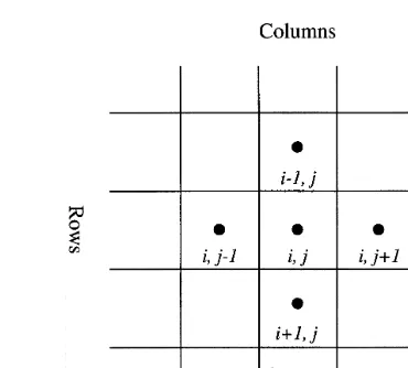
Numerical methods such as finite difference or finite element are often used in the solution of eqn (3). In this paper, the block-centered finite difference method is used,
and the regionQis discretized into a grid system as shown
on Fig. 1. Specifically, the x-direction is divided into nxþ2
equally spaced blocks with the block-centered nodal points
labeled by 0, 1,…, nx, nxþ1 where 0 and nxþ1 indicate
nodal points at the constant-head boundaries. Similarly, the
y-direction is also divided into nyþ2 equally spaced blocks
with the block-centered nodal points labeled by 0, 1,…, ny,
ny þ 1. Let nx, and ny be the number of active (interior)
nodal points in x and y coordinates axes, respectively and let
Dx andDy denote the grid spacings and hi,j¼h(jDx, iDy),
and wi,j ¼ w(jDx, iDy). Then, the governing equation as
expressed in eqn (3) is discretized as a set of difference equations:
Ki,jþ1=2
hi,jþ1¹hi,j
(Dx)2 ¹Ki,j¹1=2
hi,j¹hi,j¹1
(Dx)2
þKiþ1=2,j
hiþ1,j¹hi,j
(Dy)2 ¹Ki¹1=2,j
hi,j¹hi¹1,j
(Dy)2
þwi,j¼0 ð4Þ
where the K values at the interface between two nodal points are estimated from those at the two neighboring nodal points as follows,
Ki,jþ1=2¼
2Ki,jKi,jþ1 Ki,jþKi,jþ1
(5a)
Ki,j¹1=2¼
2Ki,jKi,j¹1 Ki,jþKi,j¹1
(5b)
Kiþ1=2,j¼
2Ki,jKiþ1,j Ki,jþKiþ1,j
(5c)
Ki¹1=2,j¼
2Ki,jKi¹1,j Ki,jþKi¹1,j
(5d)
To introduce vector notation we let m¼(i¹1)nxþj, n¼
nx•ny, hm ¼ hi,j, i ¼ 1,2,…, nx, j¼1;2;…ny and
{h}¼[h1;h2…hn]T. After rearranging the terms, the
following system of linear equations is obtained,
gm¹nxhm¹nxþcm¹1hm¹1þamhmþbmhmþ1
þdmhmþnx¼fm m¼1,2, …n ð6Þ Fig. 1. Illustration of the block-centered finite-difference grid
where
These equations can be written in a matrix form as,
A{h}¼{f } (8)
where A is a band matrix with dimension n
A¼
The above system of linear equations is often solved by
iterative methods, including successive over-relaxation14
or conjugate gradient methods.9
3 PERTURBED SOLUTIONS
In this section, we analyze the perturbed solutions for changes in the matrix A and the vector {f} . We will first consider the change in A caused by changes in hydraulic conductivity, keeping the vector {f} fixed. We will then consider the change in vector {f} due to changes in the sink/source term, holding matrix A constant. Finally, we will address the case where both matrix A and vector {f} change simultaneously. Since we deal with systems of linear equations, the solutions are additive when both A and {f} change.
3.1 Change in matrix A
To decompose the matrix we denote by {ei} the column
vector whose i-th element is one and zeros otherwise and
let Eij ¼ {ei}{ej}T denote the n by n matrix whose only
non-zero element is at location (i,j) with value one. The matrix A can now be decomposed into either column or row vectors,
From the discussion in the previous section, one can see that when the K value is changed at one location in the grid, say, location (i,j), only a small number of entries in matrix
A will be changed. Let A9 ¼ A þ DA be the changed
matrix and {h9} ¼ {h} þ {Dh} be the changed heads.
From Noble and Daniel,17 we know that if A is an n by n
nonsingular matrix, C is an n by p matrix and R is an p by
n (p,n) matrix, then the disturbed matrix A9¼AþCR is also nonsingular and its inverse is given by
(A9)¹1¼A¹1¹A¹1CZ¹1RA¹1 (11)
where Z¼IþRA¹1C is also assumed to be a nonsingular
matrix.
At first glance, eqn (11) appears to be unrelated to our
problem. However, suppose that we have A{h} ¼{f} and
A9{h9}¼{f}, and multiply eqn (11) by {f} on both sides,
we find that the new solution {h9} can be obtained from
the old one {h} as
{h9}¼{h}¹A¹1CZ¹1R{h} (12)
If p is much smaller than n, the size of Z will be much smaller than the size of matrix A, and computing inverse of matrix Z will be much easier and faster than computing the
inverse of the entire matrix A9. For example, if the value aij
in A is changed from aijto a9ij¼aijþd, then from eqn (10)
the corresponding changes are DA ¼ dEij, C¼{ei},
R¼d{ej} T
, and Z reduces to a scalar, Z¼1 þd{ejT}{b}.
Thus, the disturbed solution {h9} would be
{h9}¼{h}¹ d
1þd{eT
j}{b}
{b}{eTj}{h} (13)
wherebis the solution of A{b}¼{ei}.
In this example, to obtain the perturbed solution the system of linear equations has to be solved twice, and thus there is no advantage of using the proposed method. However, if the problem requires changing each entry in the matrix A, then multiple perturbed solutions are obtained readily by updating eqn (13).
matrix becomes A9¼AþDA where the perturbed portion
DA is given by
Recall m¼j þ(i¹1)nx. All the 13 non-zero entries are
listed in the matrix. The specific changes can be calculated
by using eqn (7). The matrix DA can be written as the
product of two smaller matricesDA¼CR where matrices
C and R are, respectively,
C¼ em¹nx em¹1 em emþ1 emþnx
with 13 non-zero entries located at
Z¼
Inversion of Z is simple and straightforward. After the inverse of Z is updated, the inverse of matrix A and
the new solution {h9} can be obtained readily from
eqns (11) and (12), respectively.
3.2 Change in vector {f}
When the sink/source term is varied at a nodal point, only
the vector {f} in equation A{h}¼{f} will be affected. Let
{h9} be the solution of A{h9} ¼ {f9} where
{f9}¼{f }þ{Df }. Since the inverse matrix B ¼ A¹1 has been saved, the new solution can be obtained immediately
by {h9}¼B{f9}¼{h}þB{Df }.
3.3 Changes in both matrix A and vector {f}
When the K values change at the boundary nodal points, both matrix A and vector {f} will be affected. Suppose that
{h0} is the solution of A9{h0} ¼{f9}. Again, we assume
A{h}¼{f} and A9{h9}¼{f}. The new solution {h0} can
be split as {h0}¼{h9}þ{Dh} and {f9} is written as {f9}¼
{f} þ {Df}. Hence, we have A9{h9 þ Dh}¼{f }þ{Df },
which yields A9{Dh}¼{Df}. Since the inverse of A9has
been updated by eqn (11) and stored, the solution {h0} can
be obtained by simply adding the two solutions {h9} and
{Dh}.
4 COMPUTATION OF THE INVERSE MATRIX B
There is an extensive literature on matrix inversion,
including George and Liu,6Duff et al.5and Press et al.18
Matrices can be inverted using either direct methods or iterative methods. Direct methods are efficient and simple when the size of the matrix is small. However, they are seldom used in large-scale systems in groundwater modeling primarily due to the computer memory requirement.
4.1 Direct methods
The inverse can be determined directly by Gaussian elim-ination or its variants. For computing the inverse of small matrices, Gaussian elimination is probably as efficient as any other method. That is, one starts with the matrix [A, I] and applies elementary row operations to change the matrix
A into the identity matrix [I, B] and the corresponding
matrix B will be the inverse. An obvious drawback of this method is that it takes twice as much memory as is needed to
store the matrix A. Press et al.18presented a routine in which
the matrix inverse B is gradually built up in A as the original
A is destroyed.
4.2 Iterative methods
Essentially, finding the inverse of matrix A is equivalent to
solving the equation AB ¼I. Iterative techniques that are
used in solving A{h}¼{f} can also be applied in finding the
inverse. Let {bi} be the i-th column of matrix B. Then one
repeatedly solves the system of equations A{bi}¼{ei}, i¼
1,…,n. Using some matrix properties that will be addressed
in the following discussions, one does not have to solve the system of equations n times.
Another use of iterative methods is to clear up numerical errors. After a number of updates of the inverse matrix required for perturbed solutions, round-off errors and other numerical errors will be accumulated in the inverse
matrix A¹1. One simple but efficient iterative algorithm can
be used that clears up these errors.8Let B0be the inverse of
A that needs to be ‘cleared’. The iterative algorithm is given
by
Bkþ1¼Bk(2I¹ABk) (18)
The algorithm stops as long as Bkþ1is close to Bk. Note that
this method can be used only when B is near the true values of the inverse. Otherwise the algorithm may not converge. How often eqn (8) needs to be applied to clear up the errors requires numerical experiments and also depends on the desired accuracy.
4.3 Storage of the inverse matrix
The memory requirement for storing the inverse matrix B grows rapidly with the size of the problem. It requires (nx,ny)2 3 NB, where NB is the number of bytes of each
entry in the matrix. For example, for a two-dimensional
flow model with a dimension of nx¼ny ¼100 and each
entry stored with a length of four bytes, then the system
memory required to store matrix B is (100 3 100)2 3
4 bytes ¼ 4 3 108bytes < 400 MB. In this subsection,
we discuss possible alternative approaches that reduce the memory requirement.
4.3.1 LU decomposition
Careful examination of the structure of matrix A reveals that
it is a block tridiagonal matrix of the form
A¼
where Diare block matrices and Tiare tridiagonal matrices.
Using LU decomposition, the matrix A can be decomposed
as a product of two matrices, A ¼LU where L is a lower
triangular matrix and U is an upper triangular one. The inverse B is equal to the product of inverse of U and L, B
¼U¹1L¹1. Inverting L and U is much easier than inverting
matrix A due to the special structure. In addition, matrices L
and U are block band matrices7given by, respectively,
L¼
where the block matrices Ui can be recursively computed
by the following procedure,
Ui¼T1
If we use the LU factorization, the system memory required
is 2nx2ny3NB, which could result in substantial savings in
memory requirements. For example, for the 100 by 100
problem considered previously, only 2 3 106 3 4 bytes
< 8 MB of system memory is required if LU is used, i.e.,
a reduction of 50 times. We need to point out that this 8 MB is just for storing the LU decomposition of matrix
A. To obtain the inverse B, it is necessary to compute B¼
U¹1L¹1. Thus, the memory savings would be realized at the
expense of longer computation time.
4.3.2 Wavelet transforms
of compressing data.3The fundamental principle of WT is that the inverse matrix B is transformed into a different domain by using a set of wavelet functions called wavelet bases. Under the new domain, many coefficients that are less significant can be neglected. Only significant coeffi-cients are stored. Since there are so many different wavelet bases, which one gives the best performance in computing time and in storage size for a matrix is problem-specific that needs to be further studied. Commonly used wavelet bases
are Daubechies bases and Meyer bases.16
WT has been applied successfully in image processing
and signal analysis19and in other applications where a
sub-stantial amount of data needs to be transferred or stored. One interesting and promising application of WT is
numeri-cal analysis proposed by Beylkin et al.1,2A larger matrix (an
integral operator) is thought of as a digital image. Suppose that the operator compresses well under a two-dimensional wavelet transform, i.e., that a large fraction of its wavelet coefficients are so small as to be negligible, then any linear system involving the operator becomes a sparse system in the wavelet bases.
4.3.3 Use of auxiliary memory
If the memory requirements are still excessive after other memory-reducing techniques have been applied, one can use auxiliary memory such as hard disks or tapes. Computa-tion of inverse of A can be broken into a number of steps. In each step, only portion of the matrix is inverted and the results are stored. For example, instead of computing AB
¼I, we can split matrix B as B1and B2, and then solve,
AB1¼I1 AB2¼I2 (23)
The identity matrix I ¼[I1 I2] can be further split into a
number of smaller portions.
5 OTHER COMPUTATIONAL CONSIDERATIONS
Reductions in computational time and system memory requirements can be achieved if one carefully implements the proposed solution procedure. We discuss some compu-tational aspects that may be helpful in implementing the proposed method. First, once the inverse of the A matrix is obtained, most of the computation time that the proposed
method spends is on updating the matrix B9¼B¹BCZ¹1RB
where Z¼IþRBC. Note that Y¼CZ¹1R is a sparse matrix
with only 25 non-zero entries. The matrix YB is also a sparse matrix containing only 5 non-zero rows. The procedure of
computing B9should start with Y, YB, and then BYB. Careful
arrangement of computational sequence can lead to a sub-stantial reduction in computation time. Second, matrix A is symmetric and so is its inverse B. Thus, not only can the required memory be halved, the time in computing and updating the inverse can also be reduced accordingly.
Golub and Van Loan7 provide more detailed information
on efficient storage and manipulation of symmetric matrices.
6 NUMERICAL EXAMPLES
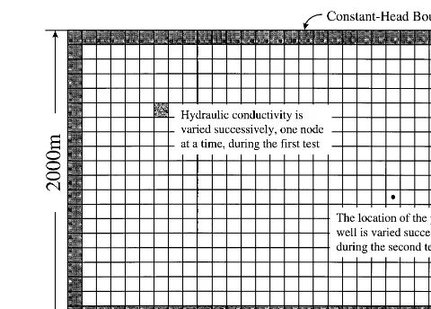
We consider a two-dimensional flow system as shown in Fig. 2. The size of the aquifer is 2000 by 3000 m. The aquifer is discretized into regularly spaced 20 rows and 30 columns. The hydraulic conductivity of the aquifer is
assumed to be constant initially with K¼100 m/day. The
head values at the specified-head boundaries are 10 m on the east, 9.1 m on the west, and on the north and south, the heads vary linearly between 10 and 9.1 m from the west border to the east border.
Two tests are conducted using the model. In the first test, the K value at one nodal point inside the boundary is changed during each model evaluation. The change of the K value is by a constant of 2 m/day. The sink/source term w is set to zero everywhere. In the second test, the K value is held constant at 100 m/day, but the w term is assigned a non-zero value sequentially at each nodal point inside the boundary during each model evaluation. With the proposed method, it is only necessary to compute the inverse matrix once. New solutions of hydraulic heads are derived on the basis of the old solution and the inverse.
The results obtained by the proposed method are com-pared with those from the finite-difference flow model,
MODFLOW.14Both methods give exactly the same
hydrau-lic heads. The standard MODFLOW code is implemented in an efficient subroutine form, eliminating all disk input/ output during successive runs. The system of linear equa-tions is solved by the Slice Successive Over-relaxation (SSOR) solver, which uses Gaussian elimination to obtain the solution in each two-dimensional ‘slice’. The test example is posed in such a way that the flow model is aligned with a slice in the SSOR procedure and the resulting system of linear equations is solved using the direct method. A new solution is recalculated by calling the MODFLOW subroutine once in response to any change in the hydraulic conductivity distribution and the sink/source term.
All computations were performed on an IBM-compatible
personal computer with a 33 mHz 80486 CPU. Table 1 presents the total CPU times (in seconds) required for the two test cases. For the proposed method, the CPU times of computing the inverse and the CPU times of updating the perturbed solutions are reported separately. The break-even number, which is the minimum number of model evalua-tions required for the proposed method to be more efficient than running the MODFLOW subroutine repeatedly, is also listed in the table. The time of updating solutions in the proposed method is so small that the break-even number can be approximated by the ratio of the time needed to invert the matrix to the time needed to obtain one solution by MODFLOW.
6.1 Test case 1: Changing hydraulic conductivity
The first example solves for the new head distribution repeatedly when the hydraulic conductivity at each model node is changed one at a time, as usually required in apply-ing a global optimization procedure such as simulated
annealing to parameter identification problems.22 For this
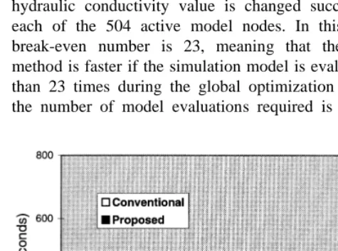
example, the numerical model is solved 504 times as the hydraulic conductivity value is changed successively at each of the 504 active model nodes. In this case, the break-even number is 23, meaning that the proposed method is faster if the simulation model is evaluated more than 23 times during the global optimization process. If the number of model evaluations required is fewer than
23, then repeatedly calling the MODFLOW subroutine is faster. The proposed method is about 15 times faster than the conventional method of calling MODFLOW repeatedly after 504 model evaluations, i.e., after the hydraulic con-ductivity value at each of the 504 active model nodes has been perturbed once. The break-even number and CPU speedup ratio depend on the problem size and the number of model evaluations required for a specific global optimi-zation procedure.
The CPU times versus the number of model evaluations are shown in Fig. 3. The CPU time required for calling MODFLOW increases linearly at approximately 0.6 s per call. In contrast, the CPU time required for the proposed method has a constant time of 14 s for matrix inversion in the first evaluation, and a much smaller time (approximately 0.01 s) for solution updating for subsequent evaluations.
6.2 Test case 2: Changing sinks/sources
The second example can be related to a remediation design problem in which the optimal locations of injection/extrac-tion wells are sought so that the total operating cost is mini-mized. In this case, the sink/source term is changed at each active model node, one node at a time, and the new heads are recalculated by using the proposed method and by call-ing the MODFLOW subroutine repeatedly. The CPU time for MODFLOW remains the same as in test case 1. How-ever, the CPU time for the proposed method decreases con-siderably because the inverse matrix does not need to be updated. It is about 19 times faster than running the MOD-FLOW subroutine repeatedly after a total of 504 model evaluations, each of which corresponds to the change of the sink/source term at one of the 504 active model nodes.
7 POSSIBLE APPLICATIONS
The discussion of the proposed method has been based on a two-dimensional steady-state flow model. However, the proposed method can be readily extended to three-dimensional and transient models, both flow and transport, as long as they are linear. For example, for a three-dimensional steady-state flow model, there are 7 non-zero diagonal lines in the coefficient matrix A. The resulting matrix Z would be a 7 by 7 matrix when the hydraulic conductivity value changes at a model cell. Inverting a 7 by 7 matrix in the three-dimensional case is as simple and
Table 1. Comparison of computational times for tests 1 and 2
Test 1 Test 2
Total number of model evaluations 504 504
Total CPU time of calling MODFLOW 310 310
Total CPU time of the proposed method 20 16
Matrix inversion 14 14
Solution updating 6 2
Break-even number 23 23
Speedup ratio for the proposed method 15.5 19.4
easy as inverting a 5 by 5 matrix in the two-dimensional case. As for two- or three-dimensional transient flow models
in which there is a system of equations, A{hk} ¼{fk} for
each time step k, more computer memory may be needed to store the inverse matrix for each of the time steps. This is
because the coefficient matrices contain the time step sizeDt
used in transient solutions. Thus, if the time step sizeDt is
not uniform, the inverse matrix needs to be stored each time step. Except for this difference, all other procedures as used in the steady-state case are directly applicable in the transient case.
The proposed method can be directly used in the frame-work of an integrated global optimization and simulation model for identification of optimal aquifer parameters. In a global optimization procedure, such as simulated anneal-ing and tabu search, the hydraulic conductivity value may be altered at only one location for each time the objective function is evaluated. Given that tens of thousands of objec-tive function evaluations may be required in an optimization
step,22a tremendous saving in computation time would be
realized by using the proposed method as opposed to run-ning the simulation code repeatedly.
The proposed method is not only beneficial to global optimization methods, but also useful for gradient based optimization methods. For example, for parameter identi-fication problems, parameter sensitivities related to the hydraulic conductivity values at observation points are evaluated by using either the adjoint-state method or the
perturbation method.10 Instead of repeatedly evaluating
the forward simulation code, the proposed method can be applied to obtain the sensitivities. If the number of observa-tions is large enough, the proposed method is expected to be much faster.
The second direct application of the proposed method is in remediation designs in which optimal well locations and pumping rates are sought so that the total capital and operating costs associated with the remedial measures are minimized. When the pumping rates and/or well locations change in a confined aquifer, the corresponding changes
in the system of linear equations A{h} ¼ {f} are limited
to the elements in vector {f} under confined flow condi-tions. The matrix A and its inverse remain unchanged. Therefore, once the inverse of A is computed, it will not be affected by the changes in well locations and pumping rates. Updating the new solution can be done readily and efficiently since the inverse matrix has been calculated and stored.
There are two limitations associated with the new pro-posed method. First, it only works for linear systems such as flow in confined aquifers. For flow in unconfined aquifers, the coefficients of the matrix A depend upon the solution {h}. As a result, the proposed method cannot be used directly. The second limitation of the proposed method is the large amount of computer memory required. It may be possible to overcome this limitation by using new, innovative techniques for array storage such as wave-let transforms.
8 CONCLUSIONS
Global optimization models are being increasingly used in groundwater remediation designs (for both well locations and pumping rates) and in parameter identification (for both parameter structures and values). Both types of appli-cations require repeated solutions of matrix equations in the form of eqn (8) for each change in the coefficient matrices. Based on the assumption that the forward simulation model is linear and that only a very small portion of the matrices are perturbed during successive simulation runs, we have presented, in this paper, a new solution methodology that is much more efficient than solving the system of equa-tions directly and repeatedly for each change in the coef-ficient matrices. The proposed solution methodology obtains the new solution as the sum of a base solution and a solution to the perturbed portion of the coefficient matrices. The computational efficiency of the proposed method arises from the fact that the solution correspond-ing to the perturbed coefficient matrices can be easily derived without solving the full system of linear equations again.
The proposed method is tested using two relatively simple examples in which the finite-difference solutions to a two-dimensional steady-state flow model are evaluated repeatedly in response to successive changes in the hydrau-lic conductivity distribution and sink/source term. The hydraulic conductivity value and the sink/source term at each of the model active nodes is perturbed one at a time, similar to that required by repeated objective function evaluations in a global optimization procedure. The test results show that the proposed method leads to a reduction in the CPU times by more than 15 times over the method of calling the simulation code repeatedly. The reduction becomes even more significant as the number of model evaluations increases. Although only a two-dimensional steady-state flow model is used in this study, the funda-mental principles can be extended to three-dimensional, transient flow and solute transport problems. The methodol-ogy can also be employed in finite element solutions. It is believed that the proposed method would make the global optimization methods computationally more competitive, thus removing the single most formidable limitation of the global optimization methods.
ACKNOWLEDGEMENTS
REFERENCES
1. Beylkin, G., Comfier, R. and Rokhlin, V., Communications on Pure
and Applied Mathematics, (1991) 44, 141–183.
2. Beylkin, B., Coifman, R. R. and Rokhlin, V., Wavelets in numerical analysis. In Wavelets and Their Applications, ed. M. B. Ruskai. Jones and Bartlett Publishers, Boston, 1992.
3. Daubechies, I., Ten Lectures on Wavelets. Capital City Press, Philadelphia, 1989.
4. Dougherty, D. E. and Marryott, R. A., Optimal groundwater manage-ment, 1. Simulated annealing. Water Resour. Res., 1991, 27(10) 2493–2508.
5. Duff, I. S., Erisman, A. M. and Reid, J. K., Direct Methods for Sparse
Matrices. Oxford Science Publications, Oxford, 1986.
6. George, A. and Liu, J., Computer Solution of Large Sparse
Positive-Definite Systems. Prentice-Hall, Englewood Cliffs, NJ, 1981.
7. Golub, G. H. and van Loan, C. F., Matrix Computations, 2nd edn. Johns Hopkins University Press, Baltimore, MD, 1989.
8. Handbook of Mathematics (in Chinese). Peoples Education Press, China, 1978.
9. Hill, M. C., Preconditioned Conjugate Gradient 2 (PCG2), a computer program for solving groundwater flow equations. US Geological Survey Open File Report 90-4048, Denver, CO, 1990.
10. Hill, M. C., A computer program (MODFLOWP) for estimating para-meters of a transient, three-dimensional, ground-water flow model using nonlinear regression. US Geological Survey Report 91-484, Denver, CO, 1992.
11. Kincaid, D. and Cheney, W., Numerical Analysis. Brook/Cole Publishing Company, Pacific Grove, CA, 1991.
12. Marryott, R. A., Dougherty, D. E. and Stollar, R. L., Optimal ground-water management, 2. Application of simulated annealing to a
field-scale contamination site. Water Resour. Res., 1993, 29(4) 847–860.
13. Mauldon, A. D., Karasaki, K., Martel, S., Long, J. C., Landsfeld, M., Mensch, A. and Vomvoris, S., An inverse technique for developing models for fluid flow in fracture systems using simulated annealing.
Water Resour. Res., 1993, 29(11) 3775–3789.
14. McDonald, M. G. and Harbaugh, A. G., A modular three-dimensional finite-difference groundwater flow model. Techniques of Water Resources Investigations of the US Geological Survey, Reston, VA, 1988.
15. McKinney, D. and Lin, M.-D., Genetic algorithm solution of ground-water management models. Water Resour. Res., 1994, 30(6) 1897–1906. 16. Meyer, Y., Wavelets and Operators, In Analysis at Urbana, ed. E. Berkson, N. T. Peck and J. Hhl. London Math. Society, Lecture Notes 137, 1989.
17. Noble, B. and Daniel, J., Applied Linear Algebra, 2nd edn. Prentice-Hall, Englewood Cliffs, NJ, 1977.
18. Press, W. H., Teukolsky, S. H., Vetterling, W. T. and Flannery, B. P.,
Numerical Recipes in FORTRAN, The Art of Scientific Computing,
2nd edn. Cambridge University Press, Cambridge, 1992.
19. Ruskai, M. B. (ed.), Wavelets and Their Applications. Jones and Bartlett Publishers, Boston, 1992.
20. Wagner, B. J., Sampling design methods for groundwater modeling uncertainty. Water Resour. Res., 1995, 31(10) 2581–2591. 21. Wang, M. and Zheng, C., Aquifer parameter estimation under
tran-sient and steady-state conditions using genetic algorithms. In
ModelCARE’96: Uncertainty and Reliability of Groundwater Models, IAHS Publication no. 237, Wallingford, UK, 1996, pp. 21–30.