CALIBRATION EVALUATION AND CALIBRATION STABILITY MONITORING OF
FRINGE PROJECTION BASED 3D SCANNERS
C. Bräuer-Burchardt, A. Breitbarth, C. Munkelt, M. Heinze, P. Kühmstedt, G. Notni Fraunhofer IOF Jena, Albert-Einstein-Str. 7, D-07745 Jena, Germany
Commission III, WG III/1
KEY WORDS: Fringe Projection, Calibration Evaluation, Epipolar Geometry, Optical 3D Measurement
ABSTRACT:
In this work a simple new method for calibration evaluation and calibration stability monitoring of fringe projection based 3D scanners is introduced. This method is based on high precision point correspondence finding of fringe projection sensors using phase values in two perpendicular directions and epipolar geometry concerning calibration data of stereo sensors. The calibration evaluation method can be applied in the measurement process and does not require any additional effort or equipment. It allows the evaluation of the current set of calibration parameters and consideration of the stability of the current calibration over certain temporal progression. Additionally, the quality of distortion correction can be scored. The behavior of three fringe projection based 3D stereo scanner types was analyzed by experimental measurements. Results of the different types of scanners show that calibration may be stable over a long time period. On the other hand, suddenly occurring disturbances may be detected well. Additionally, the calibration error usually shows a significant drift in the warm-up phase until the operating temperature is achieved.
1. INTRODUCTION
Contactless scanning of the surface of different measuring objects is increasingly required in industry and technique, scientific research, cultural heritage preservation and documentation, and in medicine. Fringe projection is the basic principle of a family of such 3D scanners. Flexibility, measuring accuracy, measurement data volume, and fields of application always increase. However, it should be guaranteed that the promised accuracy which is established theoretically can be also achieved under real measurement conditions.
High precision measuring systems based on image data require high precision optical components. The measuring accuracy, however, depends additionally on the quality of the geometric description of the components. The procedure of determination of the geometry of the optical components of a 3D scanning system is performed in the process of camera calibration. The correctness of calibration is crucial for the quality of a photo- grammetric system and essential for its measuring accuracy. The set of calibration data will be produced in the process of initial calibration in the production process of a certain 3D sensor device. However, it is usually not known how stable the initial calibration is over a longer time period. As Luhmann describes (Luhmann et al. 2006), modern photogrammetric measurement systems based on active structured light projection can achieve a measurement accuracy of up to 1:100000 compared to the length extension of the measuring field. However, such high accuracies can only be achieved, if the geometry of the measuring system is stable over the time between calibration and measurement. This is, unfortunately, only the case, if certain measurement conditions strictly hold. However, in the practical use this cannot always be ensured as e.g. reported by Hastedt (Hastedt et al. 2002) or Rieke-Zapp (Rieke-Zapp et al. 2009).
The stability of the calibration data of certain cameras which are used for measurement tasks has been recently analysed by several authors. Mitishita (Mitishita et al. 2003) analyses the interior orientation parameters from small format digital cameras using so called on-the-job-calibration. Shortis (Shortis et al. 2001) examines the calibration stability for a certain digital still camera. Läbe (Läbe and Förstner 2004) determines the geometric stability of low-cost digital consumer cameras. Habib (Habib et al. 2005) analyses the stability of SLR cameras over a long period (half a year). An interesting approach presents Gonzales (Gonzales et al. 2005) in his work. He analyses the stability of camera calibration depending on the proposed calibration technique.
2. BASIC PRINCIPLES
2.1 Phasogrammetry
Phasogrammetry is the mathematical connection of photogram- metry and fringe projection. The classical approach of fringe projection is described e.g. by Schreiber (Schreiber and Notni, 2000). It can be briefly outlined as follows. A fringe projection unit projects well defined fringe sequences for phase calculation onto the object, which is observed by a camera. Measurement values are the phase values obtained by the analysis of the observed fringe pattern sequence at the image coordinates [x, y] of the camera. The 3D coordinates X, Y, Z of the measurement point M are calculated by triangulation, see e.g. (Luhmann et al., 2006). The calculated 3D coordinate depends linearly on the phase value.
2.2 Epipolar Geometry
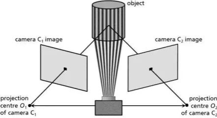
The epipolar geometry is a well-known principle which is often used in photogrammetry when stereo systems are present. See for example (Luhmann et al., 2006). It is characterized by an arrangement of two cameras observing almost the same object scene. A measuring object point M defines together with the projection centres O1 and O2 of the cameras a plane E in the 3D space (see also Figure 1). The images of E are corresponding epipolar lines concerning M. When the image point p of M is selected in camera image I1 the corresponding point q in camera image I2 must lie on the corresponding epipolar line. This restricts the search area in the task of finding corresponding points. In the following we consider a system consisting of two cameras C1 and C2 and one projector in a fix arrangement.
Figure 1: Stereo camera arrangement with fringe projector 2.3 Camera Calibration
Camera calibration is the determination of the intrinsic and extrinsic parameters (including lens distortion parameters) of an optical system. It has been extensively described in the literature, e.g. by Luhmann (Luhmann et al. 2006), Chen (Chen and Brown 2000), Brown (Brown 1971), Tsai (Tsai 1986), or Weng (Weng et al. 1992). Different principles are applied to perform camera calibration. The selection depends on the kind of the optical system, the exterior conditions, the effort to be pushed, and the desired measurement quality. In case of the calibration of photogrammetric stereo camera pairs, the intrinsic parameters of both cameras should be determined as well as the relative orientation between the cameras. Intrinsic parameters include principal length c, principal point pp = (u, v), and distortion description.
The position of the camera in the 3D coordinate system is described by the position of the projection centre O = (X, Y, Z)
and a rotation matrix R obtained from the three orientation angles (pitch angle), (yaw angle), and (roll angle). Considering stereo camera systems, only the relative orientation between the two cameras (Luhmann et al. 2006) has to be considered, because the absolute position of the stereo sensor is usually out of interest. Lens distortion may be considerable and should be corrected by a distortion correction operator D. Distortion may be described by distortion functions as e.g. proposed by Tsai (Tsai 1986), or Weng (Weng et al. 1992), or by a field of selected distortion vectors (distortion matrix), as suggested by Hastedt (Hastedt et al. 2002) or Bräuer-Burchardt (Bräuer-Burchardt et al. 2004).
3. APPROACH FOR CALIBRATION EVALUATION
3.1 Basic Assumptions
Let us consider a fringe projection based stereo scanner with two cameras and one projector in a certain arrangement (see also Figure 1). 3D surface data are aquired by a measurement from one sensor position using either epipolar constraint (mode
m1) or fringe pattern sequences in two orthogonal projection directions (mode m2 - see Schreiber and Notni, 2000). Point correspondences with sub-pixel accuracy are found using equal phase values in both camera images. Whereas using mode m2 always guarantees to find correct point correspondences, searching on epipolar lines (mode m1) leads to point correspondence errors. However, mode m1 needs half the length of the image sequence and hence image sequence recording needs half the time only.
The calibration of the sensor is performed once in the laboratory and is assumed to be fix over a longer time period. Calibration data include intrinsic and extrinsic parameters and a set of distortion parameters or a distortion matrix for each camera. Calibration may be performed again, of course, if it seems to be necessary. However, this means usually high effort. Alternatively, self-calibration (Schreiber and Notni 2000) can be performed at every measurement. However, conditions may be too poor to obtain robust parameters from self-calibration. 3.2 Goal
Especially moved sensors are susceptible to mechanic shocks and vibrations. These influences may disturb the current calibration, and calibration parameters become erroneous. Additionally, it is well known that calibration data are temperature dependent. Thermic changes in the environment or increase of working temperature of the sensor may also influence the calibration parameters.
The goal of this work is to describe the current state of the set of calibration parameters of fringe projection based stereo sensors. Small errors can be compensated by parameter correction whereas considerable errors should imply the decision to perform a new calibration.
3.3 Epipolar Line Error
Obviously the correct position of the epipolar lines strongly depends on the accurate values of the calibration data set. Therefore calibration errors directly influence the correctness of point correspondences, if searched on the epipolar lines. Hence, if corresponding points are located exactly on the corresponding
However, this is not sufficient for the statement that the calibration data are correct. Certain calibration parameters may be disturbed without having a considerable influence on the position of the epipolar lines but leading to a disparity error which leads, subsequently, to a depth error of the reconstructed 3D points. On the other hand, if the epipolar line position is erroneous, calibration data must be disturbed.
Let us consider two corresponding points pi and qi. The epipolar line position error errpos(p,q)i is defined as the perpendicular
where n is the number of considered corresponding point pairs. These points should be well distributed over the images. Additionally, the maximal epipolar line error Emax can be considered: Emax = max{ | errpos(p,q)i |}, i = 1, …, n.
Alternatively, a value of the 95% percentile may be chosen for Erms in order to prevent using outliers. Actually, epipolar line position error errpos(p,q)i is signed in contrast to rms epipolar
line error Erms. This is meaningful, because the sum of all
errpos(p,q)i may be near zero whereas the amount of rms epipolar line errorErms may be considerable.
3.4 Analysis of Calibration Parameter Error Influence
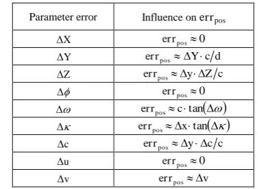
Let us consider the parameters of interior orientation ci, ui, vi, between the cameras near triangulation angle, and small roll (or rotation) angles i for both cameras. Assume X-axis alignment approximately parallel to the baseline. Estimation of the influence of erroneous calibration parameters and image co-ordinates to the epipolar line error errpos was performed. It was derived from intercept theorems and collinearity equations (see e.g. Luhmann et al. 2006). Results of error influence estimation are given in table 1, where x and y are the centered image coordinates, and d is the distance to the measuring object. A more detailed analysis of the error influence was performed by Dang (Dang et al. 2009).
3.5 Calibration Evaluation
The idea for calibration evaluation is to simply describe the calibration quality by the amount of the rms epipolar line error
according to equation (1). In order to get a significant value, representative points should be extracted being well distributed over the images. Hence, a virtual grid of image coordinates is
Table 1: Influence of calibration parameter errors for a certain aerial arrangement
3.6 Approach for Calibration Correction
The knowledge of the amount of the mean epipolar line error implies the idea to manipulate the calibration parameters such that the mean epipolar line error becomes minimal. This was performed with the help of a newly developed algorithm, which is described by the authors (Bräuer-Burchardt et al. 2011). It can be briefly explained as follows. In a first step an analysis of the influence of the single calibration parameters is performed. A reduced set of parameters with considerable and different sensitivity (see next section) is selected. The remaining parameters (in our experiments between three and seven) are systematically changed thus that a minimization of the mean epipolar line error is achieved. This will be achieved by an iterative algorithm. The manipulated parameters are now used as the current calibration data. Usually, using this method the
rms epipolar line error may be reduced to a value of near or below 0.1 (pixel). This is very accurate and allows finding point correspondences on the epipolar lines with high precision. This algorithm may be extended performing the minimization of the scaling error, too. Scaling error realizes the consideration of those parameters having a poor sensitivity to the epipolar line error (Bräuer-Burchardt et al. 2011). However, for the determination of the scaling error additional information is necessary which cannot be extracted from the phase data of an arbitrary measuring object. Here an object with well-defined lengths should be used, e.g. a grid pattern.
4. EXPERIMENTS AND RESULTS
4.1 Simulation of Calibration Parameter Error Influence
4.2 Simulation Example of a 3D Measurement
In order to illustrate the effect of an erroneous calibration parameter set simulations was performed showing a scene with four spheres with two different diameters (1 mm and 2 mm) and a frustum of a cone, respectively. 3D reconstruction was performed using original and disturbed data. The (meaningful) amount of disturbance (Erms = 1, 2, and 5, respectively) was chosen according to experimental results. See Figures 2 and 3 which illustrate the effect of disturbed calibration parameters. Considering the spheres, it can be seen that the effect of parameter errors is hardly detectable from the subjective evaluation of the sphere shape, even if the error is big (five pixel). However, decreasing completeness can be observed. Contrary, the results of the frustum of a cone imply that errors can be detected earlier by user observation.
Table 2 documents the error D of the sphere diameter measurement and the maximal length measurement error lenmx obtained by the distance measurement between two sphere centre points. Additionally, the mean standard deviation SDmn of the 3D points on the sphere surfaces is given. The size of the simulated scene was about 20 mm x 15 mm, the sphere diameters D were D1 = 1.98 mm and D2 = 3.96 mm and the distance between the spheres 11.9 and 16.8 mm, respectively. It can be seen that epipolar line error has a considerable and non-linear influence on the diameter error. Moreover, the smaller the diameter the bigger is the percentage error. Length error, however, is weak and increases proportionally.
Figure 2: Sphere measurement (simulation) with E = 0, E = 1, E = 2, andE =5 (from left to right)
Figure 3: Simulated frustum of a cone measurement with E = 0, E = 1, E = 2, andE = 5 (from left to right)
E
[pixel]
D1
[µm]
D1
[%]
D2
[µm]
D2
[%]
lenmx
[µm]
lenmx
[%]
SDmn
[µm]
- - - . - - 2,6
1 -5,4 0,27 -1,6 0,04 -2,5 0,015 2,9
-18 0,90 -3 0,08 -5 0,03 3,1
-70 3,50 -22 0,54 -12 0,07 5,0
Table 2: Influence of calibration parameter error E on measurement errors of two spheres
4.3 Experiments on Real Data
In the following a number of experiments using real sensor data are documented. The temporal course of the epipolar line error is considered using three different sensor types (see Figure 4).
The first sensor DS (see Kühmstedt et al. 2007) has a measurement field of about 20 mm x 14 mm. The image size is 516 x 778 pixel leading to a local resolution of about 35 µm. Two sensors DS1 and DS2 were analysed. The second sensor HS (see Bräuer-Burchardt et al. 2011) has a measurement field of about 50 mm x 40 mm. The image size is 2448 x 2048 pixel leading to a local resolution of 20 µm. The third sensor CS (see Munkelt et al. 2007) has a measurement field of about 240 mm x 175 mm. The image size is 640 x 474 pixel leading to a local resolution of 350 µm. Two devices CS1 and CS2 of sensor type CS were analysed.
Figure 4: Scanning devices DS (schematic image - left), HS (middle), and CS (right)
Sensors DS and CS are hand held, light weight and mobile scanners with low spatial resolution whereas sensor HS is a high resolution sensor (5 Mpixel) designed for flat measuring objects. More details are given by the authors (Kühmstedt et al. 2007, Munkelt et al. 2007, Bräuer-Burchardt et al. 2011). The measurements were performed as follows. A white nearly plane object was chosen as measurement object. Measurements of the coordinates of corresponding points of rectangular grid points well distributed over the image plane were performed using a 16 phase algorithm of orthogonally rotated phase directions. It can be assumed that the point correspondence error is negligible. For each corresponding pair of points the epipolar line position error was determined by the perpendicular distance of the measured point qi to the calculated position of the epipolar line gi. Mean epipolar line error was calculated using equation (1) and used as feature size of the calibration quality.
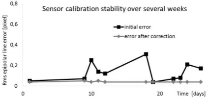
By the measurements two aspects of calibration stability should be checked. First, the stability over a longer time period (several weeks) was analysed. For this experiment evaluation measurements were selected with warmed up sensors. The result of epipolar line error of the sensor DS1 is illustrated in Figure 5.
calibration stability from switching on the device until the reaching of the operating temperature. These experiments were performed for all three scanners and repeated several times. By Figures 6 and 7 the behaviour of epipolar line error over 120 minutes of the rms epipolar line error of scanner DS is documented for two days. Decreasing error in the “warm up” phase is due to the heating up of the scanner to operating temperature of about 40°. The warming up time takes between 30 and 45 minutes.
Figure 6: Rms epipolar line error of scanner DS1 over two hours from switch on, 2011/02/07, measuring object: plane
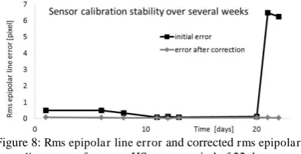
Figure 7: Rms epipolar line error of scanner DS2 over two hours from switch on, 2011/05/13, measuring object: teeth arc Sensor HS was first analysed over three weeks. See results documented in Figure 8. It can be seen that the calibration is very stable until day 20. Between day 20 and day 21 something happened which disturbed the calibration. However, correction was always possible with a remaining rms epipolar line error below 0.1 pixel.
Figure 8: Rms epipolar line error and corrected rms epipolar line error of scanner HS over a period of 22 days Next, the behaviour in the warm-up phase was checked at five days. See the results of one measurement illustrated by Figure 9. The progress of the rms epipolar line error at the other days was almost identic.
Last but not least sensors of type CS were checked. Figure 10 shows the rms epipolar line error over 30 minutes from switch on of sensor CS1. Scanner CS2 showed similar behaviour.
Figure 9: Rms epipolar line error of scanner HS over two hours from switch on, 2011/04/06, measuring object: plane
Figure 10: Rms epipolar line error of scanner CS1 over 30 min. from switch on, 2011/02/28, measuring object: plane
4.4 Detection of Erroneous Distortion Description
Epipolar line error can be also used to detect insufficient distortion correction. If correction of radial distortion is not applied correctly, this implies a certain epipolar line error. See Figure 11 which illustrates the effect of disturbed calibration parameters on the epipolar line error.
Figure 11: Effect of insufficient distortion correction of CS2: the vectors indicate epipolar line error scaled by factor ten, epipolar lines run vertically, image section is cutted above and below
5. DISCUSSION AND OUTLOOK
The three analyzed scanner types show similar behavior of the calibration quality represented by the rms epipolar line error. After being switched on the sensors need a certain time to reach their operating temperature. The duration of this warm-up phase is different depending on the properties of the sensors and can be exactly determined by the proposed method.
iterative change of between three and seven calibration parameters and minimization of the epipolar line error (Bräuer-Burchardt et al. 2011). However, it should be analyzed, whether the proposed correction is sufficient in the current case. Because only the position of epipolar lines is optimized, the corrected set of calibration parameters is only better than the erroneous one, but not really true. New calibration has possibly to be performed in the case of strongly disturbed calibration.
Future work should be addressed on the improvement of the current calibration correction procedure, the monitoring of several 3D scanners over longer periods (several months), and the fully automation of the developed algorithms so far. When scaling error can be determined, a correlation analysis of the
rms epipolar line error and scaling error should be performed. This will possibly allow a blind correction of more calibration parameters than three.
Furthermore, we plan to develop a new algorithm which realizes the correction of the calibration parameter set using an estimation of the fundamental matrix (see Zhang 1998). First attempts showed a low numeric robustness but the method should be improved.
6. SUMMARY AND CONCLUSION
In this work a simple new method for calibration stability monitoring of fringe projection based 3D scanners was introduced which allows considering the stability of the current calibration over certain temporal progression. The behavior of three types of fringe projection based 3D stereo scanners was analyzed by experimental measurements.
Only in the case of occurrence of calibration parameter errors without showing the epipolar line error effect the proposed method is not sensitive and will not detect a disturbed calibration. However, this case is very unlikely.
Calibration evaluation by the proposed method should be applied if epipolar constraint is used in order to realize point correspondences and the stability of the set of calibration parameters may be disturbed by thermic (warm-up) or mechanic (shocks or vibrations) influences. Correction is necessary according to the amount of the detected error and the requested measuring accuracy. The proposed method is ideal for determination of the end of the warm-up phase and for correction of the point correspondence in the warm-up phase.
REFERENCES
Bräuer-Burchardt, C., 2005. A new methodology for determination and correction of lens distortion in 3D measuring systems using fringe projection. In Pattern Recognition (Proc 27th DAGM), Springer LNCS, pp. 200-207
Bräuer-Burchardt, C., Breitbarth, A., Kühmstedt, P., Schmidt, I., Heinze, M., Notni, G., 2011. Fringe projection based high speed 3D sensor for real-time measurements. Proc. SPIE, Vol. 8082, 808212-1 - 808212-8
Bräuer-Burchardt, C., Kühmstedt, P., Notni, G., 2011. Error compensation by sensor re-calibration in fringe projection based optical 3D stereo scanners. accepted paper at ICIAP 2011, Proc. ICIAP, Ravenna, Springer LNCS, (in print)
Brown, D.C., 1971. Close-range camera calibration. Photogram. Eng. 37(8), 855-66
Chen, F., Brown, G.M., 2000. Overview of three-dimensional shape measurement using optical methods. Opt. Eng. 39, 10-22 Dang, T., Hoffmann, C., Stiller, C., 2009. Continuous stereo self-calibration by camera parameter tracking. IEEE transactions on image processing 18(7), 1536-1550
González, J.I., Gámez, J.C., Artal, C.G. , Cabrera, A.M.N., Stability study of camera calibration methods, 2005. CI Workshop en Agentes Fisicos, Spain, WAF'2005,
Habib, A.F., Pullivelli A.M., and Morgan, M.F., 2005. Quantitative measures for the evaluation of camera stability, Opt. Eng. 44, 033605-1 - 033605-8
Hastedt, H., Luhmann, T., Tecklenburg, W., 2002. Image-variant interior orientation and sensor modelling of high-quality digital cameras. IAPRS 34 (5), 27-32
Kühmstedt, P., Bräuer-Burchardt, C., Munkelt, C., Heinze, M., Palme, M., Schmidt, I., Hintersehr, J., Notni, G., 2007. Intraoral 3D scanner, Proc SPIE Vol. 6762, pp. 67620E-1 - 67620E-9 Läbe, T., Förstner, W., 2004. Geometric Stability of Low-Cost Digital Consumer Cameras. In Proceedings of the ISPRS Congress, Istanbul, Turkey, 528-535
Luhmann, T., Robson, S., Kyle, S., Harley, I., 2006. Close range photogrammetry.Wiley Whittles Publishing
Mitishita, E., Côrtes, J., Centeno, J., Machado, A., Martins, M., 2010. Study of stability analysis of the interior orientation parameters from the small format digital camera using on-the-job calibration. Proc ISPRS, XXXVIII, part1
Munkelt, C., Bräuer-Burchardt, C., Kühmstedt, P., Schmidt, I., Notni, G., 2007. Cordless hand-held optical 3D sensor. Proc. SPIE Vol. 6618, pp. 66180D-1
Rieke-Zapp, D., Tecklenburg, W., Peipe, J., Hastedt, H., Haig, C., 2009.Evaluation of the geometric stability and the accuracy potential of digital cameras – Comparing mechanical stabili-sation versus parameteristabili-sation. ISPRS, Vol. 64/3, 2009, 248-2 Schreiber, W. and Notni, G., 2000. Theory and arrangements of self-calibrating whole-body three-dimensional measurement systems using fringe projection technique. OE 39, 159-169 Shortis, M.R.; Ogleby, C.L.; Robson, S.; Karalis, E.M.; Beyer, H.A., 2001. Calibration modelling and stability testing for the Kodak DC200 series digital still camera. In Proceedings of SPIEVideometrics and Optical Methods for 3D Shape
Measurement, San Jose, CA, USA, January 2001; pp. 148-153
Tsai, R., 1986. An efficient and accurate camera calibration technique for 3-D machine vision. IEEE Proc CCVPR, 364-74 Weng, J., Cohen, P., Herniou, M., 1992. Camera calibration with distortion models and accuracy evaluation. PAMI(14), No 11, 965-80