*Tel.: 001-202-994-0656; fax: 001-202-994-7422. E-mail address:[email protected] (R.W. Click).
24 (2000) 1447}1479
Seigniorage and conventional taxation with
multiple exogenous shocks
Reid W. Click*
George Washington University, Department of International Business, 2023 G Street NW, Suite 230, Washington, DC 20052, USA
Received 1 January 1997; accepted 24 February 1999
Abstract
The correlation between seigniorage and conventional taxation is investigated in a dynamic optimizing model which contains three shocks (to government expenditure and to the deadweight losses associated with conventional taxation and seigniorage), asymmetric costs of adjusting revenue, and potential absence of the availability of debt. Solutions and impulse response functions from the theoretical model are used to con-struct a three-variable con-structural vector autoregression (VAR) and identify the empirical reduced-form VAR. Judged by the parameter estimates, empirical impulse response functions, forecast error variance decompositions, and historical decompositions of the time series, identi"cation is successful and the econometric results are supportive of the theoretical model. ( 2000 Elsevier Science B.V. All rights reserved.
JE¸classi,cation: E5; E6
Keywords: Seigniorage; Tax smoothing; Structural VAR models
1. Introduction
Macroeconomic applications of the theory of optimal taxation imply that marginal deadweight losses should be equated across all available tax
instruments and across time periods. Recently, these propositions have been developed in models of optimum seigniorage and conventional taxation, in which monetary and"scal policies are coordinated to minimize the total excess burden of"nancing an exogenous path of government spending. The original static model of seigniorage and conventional taxation developed by Phelps (1973) has thus e!ectively enjoyed renewed interest in the aftermath of temporal investigations of conventional taxation pioneered by Barro (1979). The recent
&traditional'model of seigniorage and conventional taxation}as developed by Mankiw (1987), Grilli (1989), Poterba and Rotemberg (1990), and Trehan and Walsh (1990)}considers the e!ects of changes in government spending under the assumption that seigniorage and conventional tax revenues are freely deter-mined in each period. In response to changes in government spending, seignior-age and conventional tax revenues optimally movein the same directionin order to equate the marginal deadweight losses of the two revenue sources. Empirical analysis has focused attention on this theoretically positive correlation. Unfor-tunately, the traditional model does not perform well since empirical results suggest that seigniorage and conventional taxation are as likely to be negatively correlated as they are to be positively correlated.
When the traditional optimum taxation model fails empirical tests, the con-clusion is usually that certain governments are acting sub-optimally. Another possibility, however, is that the optimization model under investigation is incomplete. This paper examines this alternative by developing and testing a&general'model which introduces three new features: (1) multiple sources of shocks, (2) costs associated with adjusting revenues, and (3) potential absence of the availability of debt.
First and foremost, the model in this paper explicitly considers three stochas-tic shocks } one to government expenditure, one to the deadweight losses associated with conventional taxation, and one to the deadweight losses asso-ciated with seigniorage}to determine whether governments are optimizing in the presence of multiple disturbances. The traditional model of optimum tax-ation considers only the"rst of these and implicitly assumes that there are no shocks to the deadweight losses of taxation. Trehan and Walsh (1990) introduce shocks to deadweight losses as an explanation for the residual in equations relating seigniorage and conventional taxation, and point out that this residual may therefore be correlated (positively or negatively) with seigniorage and/or conventional taxation. However, Trehan and Walsh (1990) do not develop an explanation for the shocks or consider the e!ects of the shocks on seigniorage and conventional taxation in any detail. The general model presented here therefore contains implications on how governments respond to various types of shocks, not just shocks to expenditure.
capture the idea that instantaneous changes in conventional tax revenues are more di$cult to achieve than changes in seigniorage. As noted in Poterba and Rotemberg (1990, p. 4):&Income tax schedules are often legislated several years in advance. This commitment is in part the result of time lags in the legislative process'. On the other hand,&the Federal Reserve can react quickly to changed circumstances: time lags are shorter'(p. 4). When Poterba and Rotemberg (1990) conclude that the traditional optimum seigniorage tax model generally fails empirical tests, they advance this notion as an explanation:&governments are unable to adjust the structure of taxes frequently enough to enforce the" rst-order conditions implied by optimization models'(p. 15). By introducing asym-metric adjustment costs, the model allows for gradual changes in conventional taxation over several periods compared to seigniorage.
Third, the availability of debt}which is not an issue in the traditional model
}in#uences the adjustment process. When debt is freely available, borrowing smooths revenue over time, as advanced by Barro (1979). One criticism of the traditional model, however, is that debt may be constrained in some countries. Even in some countries in which debt is available, there may be a political preoccupation focusing on the budget balance period-by-period rather than intertemporally. When debt is not available, the budget must be balanced in each period, and seigniorage optimally smooths conventional tax revenue in the presence of asymmetric adjustment costs.
1Note that the sequenceMg
tN=t/0is not a choice variable in the government's optimization problem.
In the tradition of Barro (1979), all of the recent papers on optimum seigniorage and conventional taxation}e.g., Mankiw (1987), Grilli (1989), Poterba and Rotemberg (1990), and Trehan and Walsh (1990)}assume thatMg
tN=t/0is exogenous and takeMqtNt=/0andMstN=t/0as the choice variables. This is
generally done to keep the problem tractable, which will become particularly important in this paper when identifying restrictions are imposed on the reduced-form VAR in Section 3.
impulse response functions of Section 2. Historical decompositions of the time series are used to examine correlations between seigniorage and conventional taxation depending on the various shocks. Hence, two important expository features are impulse response functions and correlation coe$cients in both theoretical and empirical dimensions. Section 6 concludes.
The existing literature examines the correlation between seigniorage and conventional taxation by estimating an intratemporal Euler equation derived from a theoretical model. This approach is fairly restrictive, however, because it does not describe the responses of di!erent taxes to various exogenous shocks. In contrast, this paper uses the structural VAR methodology precisely because it demonstrates how seigniorage and conventional taxation respond to various shocks, both contemporaneously and over time, and supports an examination of the correlation. Since the VAR is more general than the Euler equation ap-proach, it can be more illuminating. For example, even if empirical results do not con"rm theoretical implications, there is potentially interesting descriptive information on how revenues actually respond to various shocks. The main empirical"nding in this paper is that the model which includes multiple shocks outperforms the traditional model that examines only a shock to government expenditure.
2. A general model of optimum government behavior
This section develops a quadratic dynamic optimization problem for a gov-ernment acting as a welfare maximizer. The model is set up such that the Euler equations are stochastic linear di!erence equations. Using the methods of Hansen and Sargent (1998), the system of linear di!erence equations is solved for paths of the government's decision variables.
To ensure that the Euler equations are linear, all variables are expressed as ratios to national output. The government is assumed to face an exogenously determined stochastic sequence of expenditure requirements,Mg
tN=t/0, wheregtis
the ratio of government spending to output in period t. Its task is to choose plans for conventional tax revenues as a fraction of output,Mq
tN=t/0, and
seignior-age as a fraction of output,Ms
tN=t/0, that satisfy an intertemporal budget
con-straint.1 Government debt is generally permitted, denoted as a fraction of output withMd
2The seminal paper on optimum seigniorage and conventional taxation by Phelps (1973) models the government as a welfare maximizer given households that are utility maximizers and derives the deadweight losses from the e!ects of taxation on household utility. As with the recent literature on seigniorage and conventional taxation}e.g. Mankiw (1987), Grilli (1989), Poterba and Rotemberg (1990), and Trehan and Walsh (1990)}this paper assumes functional forms of the deadweight losses confronting government in order to simplify the problem in preparation for empirical work. This is clearly a short-cut approximating the alternative general equilibrium analysis, but, as pointed out in the literature, is also somewhat more general in that losses confronting the government may include collection and enforcement costs, distributional consequences of taxes, and political costs of imposing taxes. For a general equilibrium model with distorting taxes and a discussion of its complexities, see Chapter 14 of Hansen and Sargent (1998).
Thus, there are three"nancing sources at the government's disposal in each period: conventional tax revenue, seigniorage, and borrowing. The"rst two of these are associated with deadweight losses of welfare from the usual public
"nance considerations, as well as costs of adjusting revenues from period to period. The third instrument is limited by the solvency condition, an intertem-poral budget constraint which precludes perpetual debt "nance, and some borrowing costs. The government is modeled as a social optimizer in the sense that excess burdens, adjustment costs, the solvency condition, and borrowing costs are taken into account when taxes are levied.
Conventional taxation and seigniorage are associated with quadratic dead-weight losses:
(1/2)[aq2t#2¹
tqt#bs2t#2Stst], (1)
where a and b are positive coe$cients that determine the marginal excess burdens of taxation (the usual distortionary e!ects of taxes on decisions con-cerning the supply of labor or output and the demand for cash balances) and
M¹
tN=t/0 and MStN=t/0 are stochastic disturbances to deadweight losses which
re#ect the fact that raising a given amount of revenue as a fraction of output is costlier in some periods than in others.2The disturbance¹
t is a shock to the
deadweight losses of conventional tax revenues, which could represent shocks to administrative and collection costs or macroeconomic shocks that indirectly a!ect conventional tax revenues. Kenny and Toma (1997), for example, demon-strate that variation in collection costs associated with conventional taxation helps explain the temporal patterns of both conventional taxation and seignior-age. As another example,¹
tmay be higher during recessions in order to capture
the idea that the burden of taxation is higher. The disturbanceS
tis a shock to
conventional taxation than through seigniorage, b must usually be greater thana, although the magnitude of the shocksM¹
tNandMStNa!ects the analysis as
well.
In addition to the deadweight losses, the government encounters quadratic costs of adjusting conventional and seigniorage revenues represented by
1
2[c(qt!qt~1)2#k(st!st~1)2], (2)
wherecandkare positive coe$cients. These adjustment costs are introduced to capture the idea that rapid changes in conventional tax revenues are more di$cult to achieve than changes in seigniorage (k(c). The government is able to raise or lower conventional revenues, but only at a cost that increases with the magnitude of the change. This is broadly interpreted as macro-economic costs associated with temporary employment and output e!ects of tax changes, the costs of changing revenue within the existing tax infra-structure (such as the collection and enforcement bureaucracies), perhaps expanding or contracting the infrastructure, and political costs of legislating tax changes. The government is also able to raise or lower seigniorage, but once again only at a cost that increases with the magnitude of the change. This is broadly interpreted as macroeconomic costs associated with temporary employment and output e!ects of seigniorage changes, the costs of changing seigniorage within the central bank, and the political costs of altering in#ation.
Finally, borrowing is associated with quadratic costs above normal risk-free interest costs:
1
2[q(dt!dt~1)2], (3)
where q is a positive coe$cient representing borrowing costs. This might represent administrative and brokerage costs. In this paper, however, it will be used as a device to allow debt to be either freely determined or completely unavailable, although any intermediate borrowing constraint is possible. For most industrial countries with well developed"nancial markets, these borrow-ing costs are likely to be trivial (q+0). In some developing countries, however, borrowing is less likely to be available, and one way to capture this is to make it prohibitively costly (q+R).
The government's objective is to choose stochastic processesMq
t,st,dtN=t/0to
minimize the present discounted value of the welfare, adjustment, and borrow-ing costs in Eqs. (1)}(3):
E0+=
t/0
bt(1/2)[aq2t#2¹
tqt#bs2t#2Stst#c(qt!qt~1)2
#k(s
subject to the periodic budget constraint:
g
t"qt#st#dt!(1#d)dt~1 (5)
and givend
~1, an initial condition. The parameterbis the discount factor. The
parameter d is the growth rate of the outstanding debt/output ratio due to interest accrual in excess of output growth, and is assumed to be constant for simplicity. Thisdmust be positive, indicating that the real interest rate in the economy exceeds the real growth rate of the economy, in order for current debt as a portion of output to be bounded. Furthermore, note that the de"nition of
din real terms does not allow for government revenue from the erosion of the nominal outstanding debt due to in#ation. In this framework, erosion of the nominal debt is fully compensated by higher interest rates, or the debt is either indexed or denominated in foreign currencies.
The government's optimization problem can be solved using Lagrange multi-pliers. The constraints in Eq. (5) are associated with a vector multiplier process
Mj
tN=t/0. Because the constraints are required to hold in all states of the world,
these multipliers are stochastic processes. The government solves the problem by choosing stochastic processes forMq
t,st,dtN=t/0and the multipliersMjtN=t/0. The
Euler equations and the intratemporal condition from the optimization problem comprise a system of three stochastic linear di!erence equations with three unknowns (d
t,qt, andst). A solution to the system exists provided thatMqtN,MstN,
and Md
tN are of exponential order less than 1/Jb, and therefore converge to
stable values.
Rather than algebraically solving the system described, this paper makes use of the dynamic programming methods developed in Hansen and Sargent (1998). In particular, the social planning problem here takes the form of a linear-quadratic control problem known as the &discounted optimal linear regulator problem'. The MATLAB programsolvea.mprovided with Hansen and Sar-gent (1998) solves the discounted optimal linear regulator problem by iterating on the Bellman equation until converging to a solution. Programming is done by specifying the parameters of the model, so several examples are presented next: the traditional model, the general model in which debt is freely determined, and the general model in which debt is not available. Each example considers both temporary and permanent shocks as relevant extremes for persistence of the shocks, and autoregressive parameters between 0 and 1 can be handled by the model as well.
The traditional model of optimum seigniorage and conventional taxation has been concerned only with government spending shocks, so the focus is onMg
tN.
A temporary change in government spending is modeled as a shock toMg
tNthat
does not persist, so Mg
tN follows a &white noise' process with positive mean.
3In programming the traditional model in the Hansen and Sargent (1998) software,M¹
tNandMStN are nonstochastic and equal to zero, and c, k, and q are set arbitrarily small. In addition, b(1#d)"1, so there is no drift in the ratio of debt to output. The steady state equilibrium is q"(b/(a#b))gands"(a/(a#b))g. For example, whenMg
tNis assumed to have a mean of 0.30 and
b"2a, the steady state equilibrium isq"0.20 ands"0.10.
of expenditures. The impulse response functions are therefore#at lines at the magnitude of the increase in conventional taxation and seigniorage. A perma-nent change in government spending is modeled as a shock to Mg
tNthat does
persist, soMg
tNfollows a&random walk'process with positive mean. The
govern-ment will optimally not use any debt to "nance the shock, but will raise conventional taxes and seigniorage to completely"nance the increase in govern-ment spending. The impulse response functions are once again#at lines at the magnitude of the increase in conventional taxation and seigniorage. The tradi-tional model of optimum seigniorage and conventradi-tional taxation therefore re-sults in conventional tax constancy (or smoothing), as advanced by Barro (1979), along with seigniorage tax constancy (or smoothing), as advanced by Barro (1989). Furthermore, since conventional tax revenue and seigniorage are always moving in the same direction and by the same proportion, seigniorage and conventional tax revenue are optimally positively correlated.3
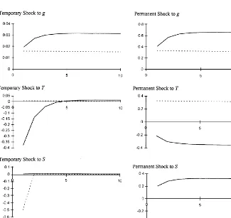
The general model allowing for multiple shocks and adjustment costs presents a richer array of possibilities than the traditional model. Fig. 1 presents impulse response functions for the general model with freely available debt, showing the e!ects of temporary shocks in the left column and the e!ects of permanent shocks in the right column. Row 1 presents the responses to government spending shocks. Note that seigniorage rises to its new equilibrium immediately because there are no adjustment costs, but conventional taxes rise gradually over several periods due to the high costs of changing conventional taxes. The di!erence between the long run equilibrium level of conventional tax revenue and the actual level of conventional tax revenue is"nanced with debt. Note also that the paths of adjustment are identical across the two shocks, but that the magnitudes (shown along the vertical axes) are di!erent because the change in the discounted present value of government spending is much smaller with a temporary shock than with a permanent shock. Row 2 shows the responses to shocks to the deadweight losses associated with conventional taxation, M¹
tN,
and row 3 shows responses to shocks to the deadweight losses associated with seigniorage,MS
tN. Note that temporary shocks cause temporary adjustments of
Fig. 1. Theoretical impulse response functions, general model with debt.
4The examples setb"2aandb(1#d)"1. As a benchmark,c"aandkis arbitrarily small. (In models of this type, the adjustment costs are usually ignored so the only costs of conventional taxation are the deadweight losses;cis therefore not likely to exceeda.) To allow debt to be freely determined,qis set arbitrarily small. Without loss of generality, the mean ofMg
tNis set to 0.30, and the means ofM¹
tNandMStNare set to zero.
5The models with and without debt represent extremes along a continuum of possibilities; for most countries, reality is probably somewhere in between.
reliance on conventional taxation (seigniorage) and increase reliance on seign-iorage (conventional taxation)by an equal magnitude, allowing for some short-run adjustments.4
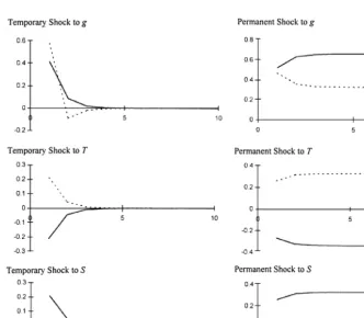
Fig. 2. Theoretical impulse response functions, general model without debt.
presents the responses to government spending shocks, row 2 shows the re-sponses to shocks to deadweight losses of conventional taxation, and row 3 shows responses to shocks to deadweight losses of seigniorage. Note that the
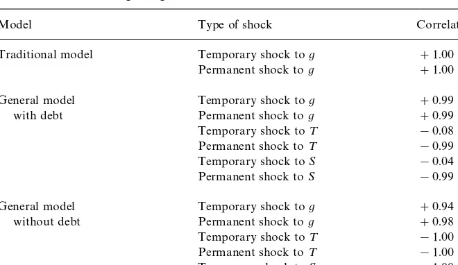
Table 1
Correlations between seigniorage and conventional taxation based on theoretical simulations
Model Type of shock Correlation
Traditional model Temporary shock tog #1.00
Permanent shock tog #1.00
General model Temporary shock tog #0.99
with debt Permanent shock tog #0.99
Temporary shock to¹ !0.08
Permanent shock to¹ !0.99
Temporary shock toS !0.04
Permanent shock toS !0.99
General model Temporary shock tog #0.94
without debt Permanent shock tog #0.98
Temporary shock to¹ !1.00
Permanent shock to¹ !1.00
Temporary shock toS !1.00
Permanent shock toS !1.00
Note: Simulations are run using the programasimul.mprovided with Hansen and Sargent (1998). The correlation is the average correlation coe$cient for 50 simulations of 100 periods each.
6To preclude debt,qis set arbitrarily high. Otherwise, the settings are the same as the ones for the model in which debt is freely available.
conventional taxation increases. The importance of seigniorage in smoothing conventional tax revenue reemerges in the examination of shocks to the dead-weight losses of conventional taxation. Conventional taxes decrease and seign-iorage increases to make up the revenue shortfall when there is a temporary shock, and seigniorage gradually approaches its equilibrium as conventional taxation gradually approaches its equilibrium when there is a permanent shock. By the nature of the balanced-budget constraint, the responses due to shocks to deadweight losses of seigniorage are exactly the opposite of the responses to shocks to deadweight losses of conventional taxation in every respect.6
In order to summarize the empirical implications of the various models and shocks, Table 1 presents correlation coe$cients between seigniorage and con-ventional tax revenue from simulations of the models. The three models are listed in the"rst column, the relevant shocks are listed in the second column, and the correlation is presented in the third column. Three major conclusions can be drawn from this table. First, there is a strong positive correlation in response to government spending shocks, regardless of the model under consid-eration. Second, permanent shocks toM¹
7For details, see Chapter 3 of Click (1994).
correlation in both the model with debt and the model without debt, because taxes are permanently recon"gured. Third, the correlation is close to zero for temporary shocks to the deadweight losses when debt is available to smooth the total revenue because only one of the two taxes is changing very much, but is strongly negative when debt is not available to smooth the total revenue because the two taxes are forced to balance the budget and are therefore forced to move in opposite directions in equal magnitudes. The main point of Table 1 is that there are theoretical reasons why conventional tax revenues and seigniorage are sometimes positively correlated, sometimes negatively correlated, and some-times uncorrelated. The models in this paper con"rm the positive correlation for cases in which the shocks come in the form of shocks to government spending. However, the models also demonstrate that conventional tax revenue and seigniorage will be uncorrelated to strongly negatively correlated if the shocks come in the form of shocks to the deadweight losses of conventional taxation and seigniorage, and that the correlation is a!ected in the case of temporary shocks by whether or not debt is available.
3. Econometric speci5cation of the model
This section develops the econometric speci"cation of the general model of seigniorage and conventional taxation. It uses solutions for paths of conven-tional tax revenues and seigniorage, along with the path of government spend-ing, to set up a three-variable structural vector autoregression (VAR). It then identi"es the structural VAR from an estimable reduced-form VAR using restrictions suggested by the model.
There are in fact several ways to approach empirical estimation of the model. In the literature on optimum seigniorage, the typical approach is to examine and estimate the Euler equations of the model in order to recover the correlation betweenq
tandst. However, initial empirical estimation of the Euler equations
8For further information on the relationship between VAR and MLE, see Chapter 8 of Hansen and Sargent (1998) or Anderson et al. (1996).
considered misspeci"ed if deadweight losses are in reality higher-order or non-linear functions ofq
tand st. (Poterba and Rotemberg (1990) and Trehan
and Walsh (1990) both assume more general constant elasticity functions.) Or, there may be short-run deviations from long-run equilibrium not captured by adjustment costs in Eq. (2). Under such circumstances, however, the structural VAR methodology will still be able to answer such questions as:&How impor-tant are the shocks?' and&How do conventional tax revenues and seigniorage respond to the shocks?'In addition, the correlation betweenq
tandstcan still be
assessed with regard to the various shocks. Maximum likelihood estimation (MLE) of the general equilibrium provides an alternative technique using the innovations representation, but would put stronger restrictions on the VAR in order to estimate the model's parameters. This may again be too restrictive if the hypothesized model is an approximation of the correct model, so this paper does not recover the deep parameters but instead estimates the dynamic multipliers (for conventional taxation and seigniorage with respect to the three exogenous shocks) which represent nonlinear functions of the deep parameters.8
Solutions to the minimization problem of Eqs. (4) and (5) express contingency plans forMq
t,st,dtN=t/0as functions of expectations of the exogenous variables Mg
t,¹t,StN=t/0and the initial conditions forq~1, s~1, andd~1. Formulations of
the contingency plans as functions of known current and past variables can be derived by specifying expectations of the exogenous variablesMg
t,¹t,StN=t/0as
functions of known current and past variables. (See the discussion of projections of geometric distributed leads in Chapter XI of Sargent (1987).)
Assume that Mg
tN,M¹tN, andMStNare orthogonal covariance stationary
pro-cesses and that expectations of future variables are linear least squares projec-tions of future variables onto information available in periodt. Consider the case in which the variables have autoregressive representations:og(¸)g
t"ugt,
o
T(¸)¹t"uTt, andoS(¸)St"uStwhereugt, uTt, anduStare white noise, andog(¸),
o
T(¸), and oS(¸) are polynomials in the lag operator. Given these processes,
there exist ARMA representations for conventional tax revenues,q
t, and
seign-iorage,s
t, such that
aq(¸)q
t"[mqg(¸) mqT(¸) mqS(¸)]R(¸)ut, (6)
a
s(¸)st"[msg(¸) msT(¸) msS(¸)]R(¸)ut, (7)
where R(¸)"diag [o
g(¸)~1oT(¸)~1oS(¸)~1], R0"I, and ut"[ugt uTtuSt]@.
The&law of motion'of the vectorx
t"[gtqtst]@is based on the autoregressive
representation for g
t and the ARMA representations for qt and st. Let
A(¸)x
The VAR representation of the structural model is therefore
[B(¸)R(¸)]~1A(¸)x
t"ut which is an estimable form, where E[utu@t]"
X"diag [u
guTuS]. The MA representation of the structural model is
there-fore:
x
t"A(¸)~1B(¸)R(¸)ut"D(¸)ut, (9)
where D0"B
0. The estimated reduced form of the VAR is represented by K(¸)x
t"gtwheregtis a 3]1 vector of white noise, E[gtg@t]"R, andK0"I.
The MA representation of the reduced form is, whereC 0"I: x
t"K(¸)~1gt"C(¸)gt. (10)
Identi"cation of the model is achieved by matching the reduced form repres-entation with the structural represrepres-entation. From Eqs. (9) and (10),
C(¸)g
Restrictions onD(¸) based on the theoretical model can thus be used to extract estimates ofD(¸) andXfrom the unrestrictedRmatrix and the MA
representa-tion,C(¸).
If the structural shocks can be modeled as unit root processes, implying that they have permanent e!ects, then the autoregressive representations of the variables are: o
where*"(1!¸). The reduced form of the VAR is therefore estimated in"rst di!erences:K(¸)*x
t"gt. Identi"cation then proceeds as in Eqs. (11)}(13).
The distinction between reduced-form VARs K(¸)x
t"gt and K(¸)*xt"gt
9In addition, if the data are di!erence-stationary but cointegrated,K(¸)x
t"gtshould be esti-mated with a cointegrating vector included, producing a vector error correction model (VECM). If some data series are stationary and other series are di!erence-stationary, mixed models should also be considered.
10For more on long-run identifying restrictions, see Shapiro and Watson (1988) and Blanchard and Quah (1989). In addition, Faust and Leeper (1997) describe some problems of long-run restrictions imposed on"nite-horizon data and suggest that short-run restrictions be taken serious-ly. For more on mixing contemporaneous and long-run restrictions, see Gali (1992).
stationary, shocks have temporary e!ects andK(¸)x
t"gtshould be estimated; if
the data are di!erence-stationary, shocks have permanent e!ects and
K(¸)*x
t"gtshould be estimated.9For the most part, the theoretical models in
Section 2 investigating temporary shocks produce temporary e!ects on conven-tional taxes and seigniorage. Although this is strictly true only for the models without debt (see Fig. 2), the permanent e!ects in the models with debt are so small that they may be approximated in empirical work by restricting them to be zero (see Fig. 1). Hence, econometric models estimated in levels can be matched against these. Since all of the theoretical models in Section 2 investigat-ing permanent shocks produce permanent e!ects on conventional taxes and seigniorage (see both Figs. 1 and 2), econometric models estimated in di!erences can be matched against them.
Identifying restrictions are required in order to extract estimates ofD(¸) and
XfromC(¸) andR. In the remainder of this section, restrictions are applied to
the long run parameters, D(1). From Eq. (13), it is evident that
C(1)RC(1)@"D(1)XD(1)@ and the twelve parameters inD(1)XD(1)@ must be
re-duced to no more than the six unique entries in C(1)RC(1)@. A just-identi"ed
system thus requires six identifying restrictions. For models estimated in levels, the long-run parameters represent cumulative responses; for models estimated in di!erences, they represent permanent responses. In addition, however, con-siderable attention is paid to the contemporaneous parameters,B
0, implied by
the long run parameters and the VAR, given by Eq. (12), B
0"C(1)~1D(1)" K(1)D(1).10
Normalizations and the exogeneity of government spending are imposed"rst. Three elements can be set through normalizations, so normalization along the diagonal in D(1) imposes D
gg(1)"DqT(1)"DsS(1)"1. Since the response of
conventional tax revenues to a shock in¹
tand the response of seigniorage to
a shock inS
tare positive under this normalization, the shocks must be
inter-preted asfavorableshocks, in contrast to the model in Section 2 where shocks are adverse. Since the theoretical model has been developed under the assump-tion that shocks to government spending are exogenous, every element in the polynomial distributed lagsD
gT(¸) andDgS(¸) is required to be zero. In
11Such restrictions identifyug, andDqg(1) andD
0. Hence, there are three normalization restrictions and two exclusion
restric-tions applied to the long-run parameters at this point. These restricrestric-tions are su$cient to exactly identify one element of X, two additional long-run
parameters, and three more contemporaneous parameters: u
g"c11,
parameters are theoretically positive, but empirical implementation does not impose this as a restriction. With the"ve restrictions applied to the long-run parameters and two additional parameters thereby exactly identi"ed, there are two unidenti"ed long-run parameters remaining (Dq
S(1) andDsT(1)). Similarly,
with one element ofXidenti"ed, there are two unidenti"ed elements remaining
(u
TanduS). Identi"cation must therefore proceed, and additional identifying
restrictions must be considered.
Additional restrictions on the elements ofD(1) are suggested by the traditional model, which does not include much of a role for shocks to¹
torSt. This could
imply either that the shocks do not exist or that the shocks do not a!ect tax-setting behavior if they do exist. The former interpretation might imply that
u
T"uS"0. However, this cannot be implemented econometrically because,
although the order conditions are satis"ed, the rank conditions are not
satis-"ed.11 The latter interpretation might imply that every element of Dq
T(¸), DsS(¸),DqS(¸), andDsT(¸) is zero, overriding the normalizations along
the diagonal. This cannot be implemented econometrically becauseD(¸) would not be invertible. However, either one of these interpretations implies that D(1)XD(1)@is singular, and this can be empirically examined by looking at the
determinant ofC(1)RC(1)@. Furthermore, feasible restrictions on theD(¸) matrix include zero restrictions on both D
qS(1) and DsT(1). This allows conventional
taxation to be a!ected by government spending shocks and conventional tax shocks, and allows seigniorage to be a!ected by government spending shocks and seigniorage shocks. This is more than the traditional model allows, but is less than the full model under consideration in this paper allows, so thus corresponds to a&generous version'of the traditional model. (Note that this in fact is not as severe as requiring every element ofDq
S(¸) andDsT(¸) to be zero,
although this would be feasible as well.) Furthermore, the restriction that Dq
S(1)"DsT(1)"0 is used for its empirical feasibility, and does not correspond
two restrictions based on a generous version of the traditional model bring the total number of restrictions to seven. Thus, there is one overidentifying restric-tion on D(1) that can be statistically tested, and is speci"cally the test of the hypothesis that Dq
S(1)"DsT(1)"0. If estimation does not fail the test of
overidenti"cation, the parameters can be examined to determine whether they appear reasonable vis-a`-vis the traditional model. If estimation fails the test of overidenti"cation, the generous version of the traditional model can be rejected based on the data.
If the exclusion restrictions based on the traditional model fail the test of overidenti"cation, further investigation based on the model with multiple shocks and adjustment costs is warranted. In particular, the zero restrictions on Dq
S(1) andDsT(1) must be dropped. Dropping one restriction or the other would
leave the VAR exactly identi"ed. However, the relationship between the two parameters can be examined following the method of Davis and Haltiwanger (1996), and this is less arbitrary and less restrictive than setting eitherD
qS(1) or
D
sT(1) to zero. The system provides a nonlinear mapping betweenDqS(1) and
D
Hence, the four unidenti"ed parameters}D
qS(1),DsT(1),uT, anduS}are jointly
determined. The method of Davis and Haltiwanger (1996) examines the sets of Dq
S(1),DsT(1),uT, anduSwhich represent solutions to the nonlinear equations
(15)}(17). Since the system is underidenti"ed, the method restricts the sets considered by simultaneously imposing qualitative restrictions on the four parameters.
SinceDq
S(1),DsT(1),uT, anduSare jointly determined, the general model with
multiple shocks can be examined by imposing qualitative restrictions on the estimated parameters that are suggested by the structural model. If there are no values ofD
qS(1),DsT(1),uT, anduSwhich simultaneously satisfy the qualitative
restrictions, the general model can be rejected, and alternative investigations might be considered. However, if there are values of D
qS(1),DsT(1), uT, and
u
values can be examined to determine whether they appear reasonable for the general model. Although the structural VAR is underidenti"ed when there are many values ofD
qS(1), DsT(1),uT, anduSwhich satisfy the qualitative
restric-tions, the four parameters can thus be identi"ed within certain intervals. The qualitative restrictions used here are sign and boundary restrictions. In particu-lar, the theory in Section 2 and the examples shown in Figs. 1 and 2 clearly indicate thatDq
S(1) andDsT(1) are the opposite signs ofDsS(1) andDqT(1),
respectively, thus providing sign restrictions. Although this is unambi-guously correct for the models when debt is not available and for permanent shocks when debt is available, it is likely to be true for the models with temporary shocks when debt is available as well. Furthermore, the model implies that the magnitudes of Dq
S(1) and DsT(1) will at most match
the magnitudes of the responses of D
sS(1) and DqT(1), respectively, thus
providing boundary restrictions. This is again evident for the models without debt and for the permanent shocks when debt is available. This lower boundary is less convincing for the models with temporary shocks when debt is available, but is useful in empirical work given that these models are estimated in levels, which forces the permanent response to be zero. Hence, two qualitative restric-tions are: !14Dq
S(1)40 and !14DsT(1)40. Since standard deviations
cannot be negative, two additional qualitative restrictions are u
T50 and
u
S50. The qualitative examination of the general model with multiple shocks
thus asks whether there are any solutions forDq
S(1),DsT(1),uT, anduSin the
nonlinear equations (15)}(17) which simultaneously satisfy these four restric-tions.
If the investigation of the long-run parameters reveals that there are values of Dq
S(1),DsT(1),uT, anduSwhich simultaneously satisfy the long-run qualitative
restrictions suggested by the structural model, an examination of the contemporaneous parameters is warranted. Since the long run parameters and the VAR imply what the contemporaneous parameters are, the appropriate-ness of the ranges for D
qS(1), DsT(1), uT, and uS can be further evaluated
using qualitative restrictions onb
qT, bsS,bsT, andbqS. Based on the theoretical
models (again see Figs. 1 and 2), four additional qualitative restrictions are available. Since Dq
T(1) andDsS(1) are both normalized to unity, shocks to
the deadweight losses of conventional taxation and seigniorage would have positive contemporaneous e!ects as well, though not exceeding the magnitude of unity. Hence, two qualitative restrictions are: 04b
qT41 and 04bsS41.
The theory also implies thatbq
Sand bsT are the opposite sign ofbsSand bqT.
Furthermore, the magnitude ofbq
Sis bounded by the magnitude ofbsSin the
model of asymmetric adjustment costs; unfortunately, no similar statement
can be made for b
sT. Hence, two "nal qualitative restrictions are:
!14!b
sS4bqS40, andbsT40. If the contemporaneous qualitative
restric-tions narrow down the ranges forD
qS(1),DsT(1),uT, anduS, identi"cation of the
4. Data and preliminary analysis
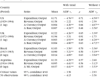
Four countries have been chosen to examine the models of seigniorage and conventional taxation: the US, the UK, Brazil, and Argentina. For the US and UK, two countries which have typically been studied in the traditional litera-ture, two measures of seigniorage are used: the change in currency and the change in the monetary base. For Brazil and Argentina, two countries which have not typically been studied in the traditional literature but for which seigniorage is generally considered more important, data are more limited. For Brazil, seigniorage is only the change in currency. For Argentina, seigniorage is the change in M1. This section characterizes the data. The"rst part describes the data and sources. The second part examines the stationarity of the series in an e!ort to determine how the VARs should be run. Section 5 then proceeds to econometrically estimate the reduced-form VARs.
The US has the highest quality data available annually for the period 1929}1994. The government spending series is total government expenditure less net interest paid, and comes from National Income and Product Accounts
(NIPA) (US Bureau of Economic Analysis). Conventional tax revenue is total tax revenue of the federal government less the transfer from the Federal Reserve to the Treasury (seigniorage), and also comes fromNIPA. Seigniorage is calculated both as the change in currency and as the change in the monetary base. Data for currency come fromHistorical Statistics of the United States(US Bureau of the Census, 1975) and are updated using theEconomic Report of the President(US Council of Economic Advisors, various issues). Data for the monetary base come from Friedman and Schwartz (1963), and are updated usingInternational Financial Statistics(International Monetary Fund, various issues). The output measure is GNP, fromNIPA.
Data for the UK are generally poorer quality than data for the US, but do exist annually for the long time horizon 1872}1990. All data series come from Mitchell (1988) and are updated usingAnnual Abstract of Statistics(UK Central Statistical O$ce). Government expenditure is reported as total expenditure and conventional tax revenue is reported as total revenue in the consolidated ac-counts. Two measures of seigniorage are again used, one as the change in currency and one as the change in the monetary base. Output is GNP at factor cost.
Data for Brazil are available for 1913}1985 on an annual basis. Total government receipts and total government expenditure come from Ludwig (1985) and are updated using Anuario Estatistico do Brasil (Ministerio da Economia). Seigniorage is the change in currency, reported as&money issued'in Ludwig andAnuario Estatistico do Brasil. The output series is GDP and comes from Mitchell (1983), and is updated usingInternational Financial Statistics.
Table 2
Augmented Dickey}Fuller (ADF) unit root tests
With trend Without trend Country
(Period) Series Mean ADFqq o ADFqk o
US Expenditure/Output 0.171 !4.76HH 0.71 !4.59HH 0.74
(1929}1994) Revenue/Output 0.158 !2.22 0.91 !2.59 0.93
(1 lag) *Currency/Output 0.004 !4.20HH 0.66 !4.07HH 0.68
*Base/Output 0.007 !4.24HH 0.48 !3.56H 0.60
UK Expenditure/Output 0.222 !4.26HH 0.85 !3.39H 0.90
(1872}1990) Revenue/Output 0.194 !3.31 0.91 !1.75 0.97
(1 lag) *Currency/Output 0.003 !4.93HH 0.49 !4.28HH 0.55
*Base/Output 0.004 !4.80HH 0.63 !4.72HH 0.65
Brazil Expenditure/Output 0.103 !3.58H 0.70 !3.36H 0.74
(1913}1985) Revenue/Output 0.090 !5.21HH 0.50 !5.19HH 0.50
(0 lags) *Currency/Output 0.014 !4.09H 0.63 !3.94HH 0.65
Argentina Expenditure/Output 0.133 !4.29HH 0.57 !2.60 0.81
(1914}1984) Revenue/Output 0.095 !4.41HH 0.56 !3.12H 0.75
(0 lags) *M1/Output 0.037 !4.41HH 0.55 !3.53H 0.70
Critical values 95% con"dence level !3.50 !2.93 50 observations 99% con"dence level !4.15 !3.58 Critical values 95% con"dence level !3.45 !2.89 100 observations 99% con"dence level !4.04 !3.51 Note:Hdenotes signi"cant at 5% level,HHdenotes signi"cant at 1% level.
12The tests are discussed in Dickey and Fuller (1979). The critical values at the 5% and 1% levels, based on tables 8.5.1 and 8.5.2 of Fuller (1976), are shown at the bottom of the table.
reported as national government revenues and exclude social security revenues. Seigniorage is the change in M1, obviously an overestimate because the govern-ment does not reap revenue in this magnitude. Due to data limitations, however, this measure is assumed to be some constant multiple of the government's true seigniorage. The measure of output is GDP at factor cost.
Table 3
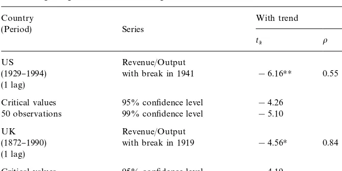
Perron}Vogelsang unit root tests allowing structural break
Country With trend
(Period) Series
t
a8 o
US Revenue/Output
(1929}1994) with break in 1941 !6.16HH 0.55
(1 lag)
Critical values 95% con"dence level !4.26 50 observations 99% con"dence level !5.10
UK Revenue/Output
(1872}1990) with break in 1919 !4.56H 0.84
(1 lag)
Critical values 95% con"dence level !4.19 100 observations 99% con"dence level !4.91 Note:Hdenotes signi"cant at 5% level,HHdenotes signi"cant at 1% level.
13The unit-root tests allowing for an endogenously-determined structural break are discussed in Perron and Vogelsang (1992). The test regression implemented here is the innovational outlier model in Eq. (7) of their paper. As recommended by Perron and Vogelsang after considering di!erent ways of selecting the order of the appropriate autoregression, the number of lags has been chosen by a test of signi"cance of the last included lag, denotedk"k(t) in their paper. The critical values at the 5% and 1% levels, based on Table 4 of Perron and Vogelsang (1992), are shown at the bottom of the table.
14I am grateful to an anonymous referee for suggesting this line of inquiry.
of World War II, and a structural change in 1941 produces the highest value of at-statistic on the shift variable. A Perron}Vogelsang unit root test allowing for an endogenously-determined structural break in 1941 is therefore presented in Table 3.13 Based on this test, the hypothesis of a unit root can be rejected in favor of the alternative hypothesis of stationarity around a changing mean.14
Hence, the conclusion is that all series for the US are stationary, once allowing for a structural break in the ratio of conventional tax revenues to output.
15For comparison, mixed models for the US and UK in whichg
tandStare temporary shocks but
¹
tis always a permanent shock have also been estimated by putting the"rst di!erence ofqtin the VAR along with the levels ofg
tandst. However, these mixed models do not improve the estimation of the VAR as much as allowing for one permanent change in theqtseries and interpreting all other changes as temporary, so the results are not reported.
mean. Hence, the conclusion is that all series for the UK are stationary, once allowing for a structural break in the ratio of conventional tax revenue to output.
Unit root tests for Brazil and Argentina more clearly reject the hypothesis of a unit root. The data for Brazil reject the null hypothesis of a unit root for all series, and are therefore considered stationary. The data for Argentina reject the null hypothesis of a unit root in all series when a trend is included. Since the trends are statistically signi"cant, all series are therefore considered stationary. On the whole, the unit root tests suggest that the data series are stationary (allowing for structural breaks in the US and UK ratios of conventional tax revenue to output). This conclusion in turn suggests that the shocks are tempor-ary (except for the single permanent changes in the US and UK ratios of conventional tax revenue to output) and that the VARs should be estimated in levels. As a result, no further consideration of models estimated in di!erences or of cointegration among variables is necessary.15
5. Empirical results
The econometric speci"cation developed in Section 3 is here applied to the annual data for the US, UK, Brazil, and Argentina described in Section 4. The strategy is to"rst examine the parameters that are exactly identi"ed by the normalization and exogeneity restrictions and to test the overidentifying restric-tions suggested by the generous version of the traditional model (Table 4), then to subsequently estimate parameter intervals based on the general model for the VARs which fail the test of overidenti"cation (Tables 5 and 6). Finally, we examine the impulse response functions for the most successful VARs (Fig. 3), and correlations between seigniorage and conventional taxation for historical decompositions of the time series (Table 7).
The VARs have been estimated in levels, and the equations include constants and logarithmic time trends. Models for the US and UK also include dummy variables to allow for the structural shifts uncovered for 1941 and 1919, respec-tively. All of the VARs impose exogeneity of government expenditure, as indicated by matricesA(¸) andB(¸).
Table 4
Parameter estimates based on overidenti"ed model Country Seigniorage LR test D
qg(1) Dsg(1)
(Period) measure (p-value) (s.e.) (s.e.) b
gg bqg bsg Jug JuT JuS
US *Currency/ 70.576 0.2464 !0.0135 0.53 0.00 0.01 0.0512 0.0149 0.0047 (1929}1994) Output(H) (0.000) (0.037) (0.012)
(4 lags) *Base/ 45.653 !0.1556 !0.1651 0.53 !0.01 0.02 0.0512 0.0234 0.0141 Output (0.000) (0.058) (0.035)
UK *Currency/ 2.196 0.4792 0.0090 0.18 0.01 0.00 0.2464 0.0527 0.0047
(1872}1990) Output(H) (0.138) (0.020) (0.002)
(4 lags) *Base/ 0.511 0.4910 0.0103 0.18 0.01 0.00 0.2464 0.0511 0.0070 Output (0.474) (0.020) (0.003)
Brazil *Currency/ 55.704 0.6141 0.1598 0.33 0.13 0.03 0.0371 0.0230 0.0188 (1913}1985) Output(H) (0.000) (0.074) (0.060)
(2 lags)
Argentina *M1/ 69.237 0.5524 0.2380 0.53 0.13 0.15 0.0337 0.0184 0.0457 (1914}1984) Output (H) (0.000) (0.066) (0.164)
(2 lags)
Note: Asterisk denotes VAR for which impulse response functions are presented in Fig. 3. Standard errors are determined using the likelihood-based function described in Section 8.5 of Doan (1992).
Click
/
Journal
of
Economic
Dynamics
&
Control
24
(2000)
1447
}
1479
Table 5
Interval estimates based on general model
Country Range of Range of Range of Range of
(Period) Seigniorage measure D
(4 lags) *Base/Output None None None None
UK *Currency/Output(H) 0 0 0.0527 0.0047
(1872}1990) *Base/Output 0 0 0.0511 0.0070
(4 lags)
Argentina *M1/Output(H) !0.32,
!0.23
Note: Asterisk denotes VAR for which impulse response functions are presented in Fig. 3.&none' signi"es that long-run restrictions cannot be satis"ed.
16In overidenti"ed VARs,D(1)JXdoes not precisely factorC(1)RC(1)@. The test of the overiden-tifying restriction is ¸R"n[ln(det(D(1)XD(1)@))!ln(det(C(1)RC(1)@))] where n is the number of observations andD(1) is restricted such thatDqS(1)"D
sT(1)"0. Exogeneity of government spend-ing is imposed in both the restricted model and the unrestricted model, soDqg(1) andD
sg(1) are the same in both. Hence, the likelihood ratio tests the hypothesis thatDqS(1)"D
sT(1)"0 against the alternative that there is a mapping betweenD
qS(1) andDsT(1).
invertible, immediately suggesting that the traditional model is inadequate. The formal likelihood ratio test (LR Test) of overidenti"cation, which is distributed
s2(1), also enables us to reject the generous version of the traditional model in most cases.16For the US, Brazil, and Argentina, there are strong rejections of the overidentifying restriction. For the UK, however, the overidentifying restric-tion cannot be rejected.
Table 4 also presents values ofD
qg(1) andDsg(1) along with standard errors.
Thus, statistical tests of the hypotheses that D
qg(1)'0 and Dsg(1)'0 can be
performed. Values of b
gg, bqg, andbsgimplied by the long run parameters are
presented as well, and the last three columns provide values ofJu
g, JuT, and
JuS. For the US, some estimates ofDq
g(1) andDsg(1) have the wrong sign. Of the
Table 6
Intervals of contemporaneous parameters based on intervals identi"ed in Table 5
Country Range of Range of Range of Range of
(Period) Seigniorage measure b
(4 lags) *Base/Output None None None None
UK *Currency/Output(H) 0.22 0.02 !0.57 0.76
(1872}1990) *Base/Output 0.23 0.00 !0.09 0.55
(4 lags)
Note: Asterisk denotes VAR for which impulse response functions are presented in Fig. 3.&None' signi"es that long-run restrictions cannot be satis"ed.
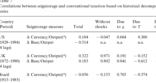
Table 7
Correlations between seigniorage and conventional taxation based on historical decompositions of series
US *Currency/Output(H) 0.104 !0.047 0.664 0.306 0.005
(1929}1994) *Base/Output !0.514 n.a. n.a. n.a. n.a.
(4 lags)
UK *Currency/Output(H) 0.322 0.971 0.191 !0.152 !0.482
(1872}1990) *Base/Output 0.183 0.802 0.041 !0.612 !0.201 (4 lags)
Brazil *Currency/Output(H) !0.056 !0.153 0.765 !0.574 !0.286 (1913}1985)
(2 lags)
Argentina *M1/Output(H) 0.224 0.997 0.871 !0.312 !0.988
(1914}1984) (2 lags)
17D
qg(1),Dsg(1),bgg,bqg,bsg, andJugare exactly identi"ed in the same manner as in Table 4.
positive and the response of seigniorage is, although negative, insigni"cant. Speci"cally, a one point temporary increase in the ratio of government expendi-ture to output originates as a 0.53 point increase and has a cumulative one point increase resulting from an autoregressive process. Although there is no contem-poraneous response of conventional taxation (implying that the entire amount is
"nanced with debt), the cumulative increase in government spending is"nanced 25% with an increase in taxes, leaving 75% to be"nanced with debt. For the UK, estimates ofDq
g(1) andDsg(1) are all positive and signi"cant. A one point
increase in government spending originates as a 0.18 point increase. Although there is a very small (0.01 point) increase in conventional taxes contempor-aneously, the cumulative increase in government spending is eventually"nanced 48% with taxes (based on the VAR using currency) and 1% with seigniorage, and therefore 51% with debt.
For Brazil and Argentina, the results in Table 4 also indicate thatD
qg(1) and
D
sg(1) are positive and usually signi"cant (the exception beingDsg(1) in
Argen-tina). In Brazil, a one point increase in government spending originates as a 0.33 point increase. Conventional taxes rise 0.13 points and seigniorage rises 0.03 points contemporaneously, leaving 0.17 points to be"nanced with debt. Cumu-latively, conventional taxes rise 0.61 points and seigniorage rises 0.16 points, leaving 0.23 points to be"nanced with debt. In Argentina, a one point increase in government spending originates as a 0.53 point increase, and is contempor-aneously"nanced with a 0.13 point increase in taxes and a 0.15 point increase in seigniorage, leaving 0.25 points"nanced with debt. Cumulatively, the one point increase in government spending is"nanced 55% with taxes, 24% with seignior-age, and 21% with debt. Based on these results and the time periods involved, Brazil and Argentina may therefore not have as much access to borrowing as the US and the UK in order to"nance temporary shocks. (For Argentina, however, recall that the measure of seigniorage is the change in M1 and this may overstate the revenues.)
Table 4 also contains estimates of the standard deviations of shocks to the systems. The values ofJu
g suggest that government spending shocks are the
most important in the UK, followed distantly by the US. The values of
JuTsuggest that shocks to the deadweight losses of conventional taxation are the most important in the UK, and the values ofJu
Ssuggest that shocks to the
deadweight losses of seigniorage are the most important in Argentina. For the US, Brazil, and Argentina, interval identi"cation ofDq
S(1) andDsT(1)
is particularly important given strong rejections of the overidentifying restric-tion. Table 5 presents ranges for the parameters which simultaneously satisfy the qualitative restrictions: !14D
qS(1)40,!14DsT(1)40,uT50, and
18VARs imposing only contemporaneous restrictions have been investigated for all of these models. Results produce estimates ofbqgandb
sgwith large standard errors and estimates ofbqSand
b
sTwhich fall in large intervals.
and conventional taxation is a potentially important description of government behavior. For the US, the VAR using currency does contain intervals which satisfy the qualitative restrictions. With respect to the monetary base, even taking the negative coe$cients on Dq
g(1) and Dsg(1) as given, there are no
intervals which can simultaneously satisfy the qualitative restrictions. Hence, we e!ectively reject the general model when qualitatively tested using the monetary base, but cannot reject the general model when using currency. For Brazil and Argentina, each VAR contains parameter values which satisfy the qualitative restrictions. For the US, Brazil, and Argentina, then, the general model of seigniorage and conventional taxation is promising, and identi"cation can proceed.
Table 6 presents intervals for the contemporaneous parameters which corres-pond to the intervals for cumulative parameters and standard deviations pre-sented in Table 5. For most of the VARs, contemporaneous restrictions are typically satis"ed. In particular, the qualitative restrictions onb
qTandbsSare
always satis"ed. The qualitative restriction on b
qS can be satis"ed, but is
automatically satis"ed only for the UK and Argentina. Finally, the qualitative restriction on b
sT can be satis"ed for Brazil and Argentina but cannot be
satis"ed for the US and the UK. However, even when the restriction on b
sTcannot be satis"ed, it is nearly satis"ed, which is therefore not too damaging
considering that contemporaneous parameters are generally less precisely esti-mated in these VARs and probably represent short run deviations from equilib-rium not accounted for by adjustment costs.18Overall, the fact that qualitative restrictions are generally satis"ed is evidence that the model with multiple shocks and adjustment costs may characterize the data.
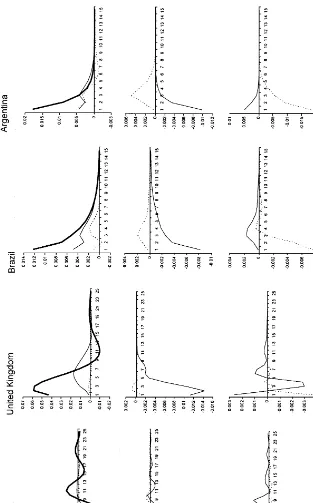
Impulse response functions from the most successful model for each country are presented in Fig. 3. For the UK, the model imposingD
qS(1)"DsT(1)"0 is
used. For the other countries, models which rejected the overidentifying restric-tion use a value ofD
qS(1) chosen to satisfy as many contemporaneous
restric-tions as possible. Shocks to¹
tandSthave been converted intoadverseshocks so
that the empirical impulse response functions can be directly compared to the theoretical impulse response functions in Figs. 1 and 2.
For the US, impulse response functions for the VAR estimated using currency are presented. Speci"cally, Dq
S(1)"!0.95, which sets DsT(1)"!0.22,
bq
T"0.48,bsT"0.02,bqS"!0.01, andbsS"0.45. Hence, onlybsTviolates its
Fig.
3
.
E
mpi
rical
im
pu
ls
e
res
p
o
nse
fu
n
ct
io
n
19For a related model of taxes and government spending without seigniorage, see Braun (1994).
to dip below zero then rise slightly above zero before settling at zero. This pattern resembles the path of government spending after the shock, but revenues are also much smoother than the path of government spending after the shock, and is therefore supportive of the optimization model. The response of seignior-age also seems to follow this pattern, but is small (and may be statistically insigni"cant based on D
sg(1)). The responses to shocks to deadweight losses
oscillate a bit much, but otherwise have appropriate patterns: in response to a shock to the deadweight loss of conventional taxation (seigniorage), conven-tional tax (seigniorage) revenues are generally lower and seigniorage (conven-tional taxation) is generally higher. Forecast error variance decompositions demonstrate that changes in conventional taxation are due 47% toM¹
tN, 52% to
Mg
tN, and less than 1% to MStN at the "ve year horizon. The decompositions
demonstrate that changes in seigniorage are due 22% toMS
tN, 48% toMgtN, and
30% to M¹
tN at the "ve year horizon. Hence, the variance decompositions
demonstrate that all three shocks are important, so the traditional model considering only shocks to government spending is inadequate. Together, the impulse response functions and the variance decompositions support the model with multiple shocks and adjustment costs, particularly because of the introduc-tion of shocks to deadweight losses of convenintroduc-tional taxaintroduc-tion.19
For the UK, either model could be used, so responses for the VAR using currency are presented for consistency. Recall that Dq
S(1)"DsT(1)"0. This
corresponds tobq
T"0.22,bsT"0.02, bqS"!0.57, andbsS"0.76. Of
particu-lar interest is the fact that the responses of seigniorage and conventional taxation to shocks a!ecting their own deadweight losses are perfectly appropri-ate. In addition, b
sT violates the qualitative restriction (because it should be
negative), but again is not too far o!, and is not surprising given thatD
sT(1)"0.
As with the US, there is gradual adjustment of conventional tax revenue after a shock to government spending, and this time the path of seigniorage is appropriate and supportive of the general model becauseD
sg(1) is statistically
signi"cant. Once again, responses to shocks to deadweight losses also have the appropriate patterns overall. Variance decompositions again suggest that all three shocks are important. Forecast error variance decompositions demon-strate that changes in conventional taxation are due 41% toM¹
tN, 57% toMgtN,
and 2% toMS
tNat the"ve year horizon. Decompositions also demonstrate that
changes in seigniorage are due 53% toMS
tN, 36% toMgtN, and 11% toM¹tNat the
"ve year horizon. Hence, although the hypothesis that Dq
S(1)"DsT(1)"0
For Brazil, the VAR again uses currency. Speci"cally,D
qS(1)"!0.50, which
setsD
sT(1)"!0.38,bqT"0.38,bsT"!0.004,bqS"!0.0001, andbsS"0.53.
Hence, all qualitative restrictions are satis"ed simultaneously. The impulse response functions in Fig. 3 also show generally appropriate paths. In response to a government spending shock, both sources of revenue increase sharply (rather than gradually as in the US and UK) and gradually return to their equilibria, a pattern resembling the model with debt constraints. Responses for shocks to¹
tandStdepict general movement in opposite directions followed by
gradual adjustment to equilibrium, somewhat resembling the model with debt, yet somewhat resembling the model without debt. Forecast error variance decompositions demonstrate that changes in conventional taxation are due 57% to M¹
tN, 38% to MgtN, and 5% to MStN at the "ve year horizon. The
decompositions demonstrate that changes in seigniorage are due 82% toMS
tN,
8% toMg
tN, and 9% toM¹tNat the"ve year horizon. Overall, the model with
multiple shocks, adjustment costs, and some debt constraints probably charac-terizes the data well.
For Argentina, all contemporaneous and long run qualitative restrictions are again simultaneously satis"ed, and the midpoint of the feasible range sets Dq
S(1)"!0.235, DsT(1)"!0.98,bqT"0.64,bsT"!0.03, bqS"
!0.13, andb
sS"0.47. The impulse response functions strongly resemble those
from the theoretical model without debt. In response to a government spending shock, both sources of revenue increase, and conventional taxes return to their initial level gradually as seigniorage drops below its initial level and approaches equilibrium from the opposite side. Responses for shocks to¹
t andSt depict
movement in opposite directions followed by adjustment to equilibrium. Fore-cast error variance decompositions demonstrate that changes in conventional taxation are due 54% toM¹
tN, 30% to MgtN, and 16% to MStNat the"ve year
horizon. The decompositions demonstrate that changes in seigniorage are due 83% toMS
tN, 9% toMgtN, and 8% toM¹tNat the"ve year horizon. Overall, once
again, the model with multiple shocks, adjustment costs, and debt constraints characterizes the data well.
To further examine the empirical models under consideration, Table 7 pres-ents correlations between seigniorage and conventional taxation for historical decompositions of the conventional tax and seigniorage series using the
identi-"cation techniques implemented for the impulse response functions. The column
&Total'presents the correlations for the raw data. The column&Without Shocks'
Weak correlations for the UK are surprising given the good results in the parameter estimates and the impulse response functions, but probably re#ect generally lighter use of both taxes (and more reliance on debt) compared to Brazil and Argentina. Table 1 suggested that the correlations due to shocks to ¹
tandStshould be near zero to highly negative depending on the availability of
debt. Except in the US, where seigniorage has already been shown to be less important, the empirical correlations"t into this range. Taken as a whole, the results in Table 7 suggest that identi"cation has been successful, particularly for the UK, Brazil, and Argentina, and that the model of optimum seigniorage and conventional taxation performs well once di!erent sources of shocks are taken into account.
6. Conclusion
This paper studies how governments"nance exogenous shocks in order to determine how seigniorage and conventional taxation covary. The theoretical part of the paper develops a model of public"nance in which there are multiple shocks, asymmetric costs of adjusting revenue, and borrowing costs that capture the possibility that debt may be constrained. As with the traditional model of optimum taxation, seigniorage and conventional tax revenues are positively correlated when the important shocks are to government spending. However, the theoretical model also introduces shocks to deadweight losses associated with both forms of taxation, and in turn suggests that seigniorage and conven-tional tax revenue will be uncorrelated to highly negatively correlated when the important shocks take these forms. The addition of asymmetric costs of adjust-ing revenues suggests that there may be important short run deviations from long run equilibrium which alter the correlations. Furthermore, this makes the availability of debt a much more important issue than previously thought, because debt smooths conventional tax revenue when it is available but seign-iorage smooths conventional tax revenue when debt is not available.
Solutions and impulse response functions from the theoretical model are used to construct a three-variable structural VAR (in government expenditure, con-ventional tax revenue, and seigniorage) and identify the structural VAR from an estimable reduced-form VAR. The theory asserts how governments optimally respond to shocks, and the empirical work examines the theory by determining whether the data can be characterized by any form of the model. Some aspects are statistically testable } such as whether Dq
g(1)'0 and Dsg(1)'0, and
whether Dq
S(1)"DsT(1)"0 } and some aspects are qualitatively examined
} such as whether !14D
qS(1)40,!14DsT(1)40, uT50, and uS50
run restrictions is successful and the econometric results support the theoretical model. The main empirical"nding is that the model which includes multiple shocks outperforms the traditional model that examines only a shock to govern-ment expenditure. For the US, Brazil, and Argentina, a generous version of the traditional model is rejected, based on tests of overidenti"cation, in favor of the more general model. Based on di$culty identifying a model for the US and the results of that model, however, seigniorage does not appear to be very important and might be appropriately left out of the public"nance analysis. Despite being unable to reject the generous version of the traditional model, the VARs for the UK provide support for the general model because of the appropriate use of seigniorage and appropriate responses of seigniorage and conventional taxation to shocks a!ecting their own deadweight losses. Models for Brazil and Argentina are indicative of the general model with multiple shocks with some debt constraints. Taken together, the chief contribution of examining these varied cases is in demonstrating the importance of multiple exogenous shocks.
Acknowledgements
This is a revised and shortened version of Chapter 2 of Click (1994). I am grateful for guidance in this research from Robert Z. Aliber, Steve J. Davis, Guillermo Mondino, and Anil Kashyap, and for comments from Brad Barber, Josh Coval, and seminar participants at Brandeis University. I am also grateful for "nancial support from the University of Chicago Graduate School of Business, the Richard D. Irwin Foundation, and the ITT Corporation.
References
Anderson, E.W., Hansen, L.P., McGrattan, E.R., Sargent, T.J., 1996. Mechanics of forming and estimating dynamic linear economies. In: Amman, H.M., Kendrick, D.A., Rust, J. (Eds.), Hand-book of Computational Economics, vol. I. North-Holland, Amsterdam, pp. 171}252. Barro, R.J., 1979. On the determination of public debt. Journal of Political Economy 87, 940}971. Barro, R.J., 1989. Interest-rate targeting. Journal of Monetary Economics 23, 3}30.
Braun, R.A., 1994. Tax disturbances and real economic activity in the postwar United States. Journal of Monetary Economics 33, 441}462.
Blanchard, O.J., Quah, D., 1989. The dynamic e!ects of aggregate demand and supply disturbances. American Economic Review 79, 655}673.
Click, R.W., 1994. Seigniorage and conventional taxation: an international investigation, Ph.D. Dissertation, The University of Chicago.
Davis, S.J., Haltiwanger, J., 1996. Driving forces and employment#uctuations: New evidence and alternative interpretations. National Bureau of Economic Research Working Papers Series No. 5775.