ISE 2: PROBABILITY and STATISTICS
Lecturer
Dr Emma McCoy,
Room 522, Department of Mathematics, Huxley Building. Phone: X 48553
email: [email protected] WWW: http://www.ma.ic.ac.uk/∼ejm/ISE.2.6/ Course Outline
1. Random experiments
2. Probability
• axioms of probability
• elementary probability results • conditional probability
• the law of total probability • Bayes theorem
3. Systems reliability
4. Discrete random variables
• Binomial distribution • Poisson distribution
5. Continuous random variables
• Exponential distribution • Normal distribution
6. Statistical Analysis
• Point and interval estimation
7. Reliability and hazard rates
Textbooks
1
Introduction – Random experiments
In general a statistical analysismay consist of:
• Summarization of data.
• Prediction.
• Decision making.
• Answering a specific question of interest.
We may view a statistical analysis as attempting to separate the signal in the data from thenoise.
The accompanying handout of datasets gives two examples of types of data that we may be interested in.
1.1
Methods of summarizing data
Dataset 1
We need to find a simple model to describe the variability that we see. This will allow us to answer questions of interest such as:
• What is the probability that 3 or more syntax errors will be present in another module?
Here the number of syntax errors is an example of adiscrete random variable
– it can only take one of a countable number of values. Other examples of discrete random variables include:
• No of defective items found when 10 components are selected and tested.
Can we summarize dataset 1 in a more informative manner ?
Frequency Table:
NUMBER OF ERRORS FREQUENCY PROPORTION
0 14 0.467
1 10 0.333
2 4 0.133
3 2 0.067
>3 0 0.0
TOTAL 30 1.0
So referring to the question of interest described above the observedproportion of 3 or more syntax errors is 0.067. This is an estimateof the ‘true’ probability. We envisage an infinite number of modules – this is the population. We have obtained a sample of size 30 from this population. We are really interested in the population probability of 3 or greater syntax errors.
We are interested in finding those situations in which we can find ‘good’ estimates.
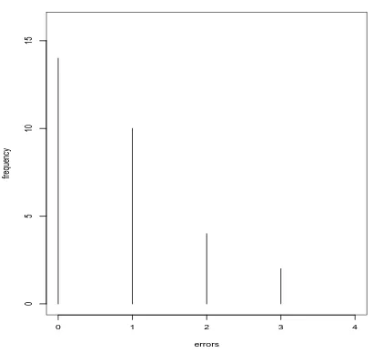
Frequency diagram (bar chart)
A frequency diagram provides a graphical representation of the data. If we plot the proportions against number of syntax errors then we have an estimate
errors
frequency
0 1 2 3 4
0
5
10
15
Figure 1: Frequency diagram for dataset 1
Dataset 2
Each value is a realization of what is known as acontinuous random variable. One assumption we may make is that there is no trend with time. The values change from day to day in a way which we cannot predict – again we need to find amodelfor the downloading time. For example we assume that the downloading times are in general close to some value µ but there is some unpredictable variability about this value which produces the day-to-day values. The way such variability is described is via aprobability distribution. For example we may assume that the day-to-day values can be modelled by a probability distribution which is symmetric about µ. We then may wish to estimate the value of µ.
Questions of interest here may include:
• What sort of spread around the average value would we expect ?
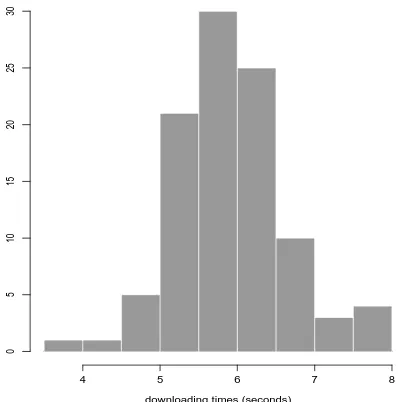
We can summarize the data more informatively using a histogram.
A histogram is simply a grouping of the data into a number of boxes and is an estimateof the probability distribution from which the data arise.
This allows us to understand the variability more easily – for example are the data symmetric or skewed? Are there any outlying (or extreme) observations?
4 5 6 7 8
0
5
10
15
20
25
30
downloading times (seconds)
Figure 2: Histogram of Dataset 2
1.2
Summary statistics
X
PROBABILITY DENSITY
-3 -2 -1 0 1 2 3
0.0
0.1
0.2
0.3
0.4
Figure 3: Normal distribution
X
PROBABILITY DENSITY
0 2 4 6 8 10
0.0
0.2
0.4
0.6
Suppose thatnmeasurements have been taken on the random variable under consideration (eg number of syntax errors, downloading time).
Denote these measurements by x1, x2, . . . , xn. So x1 is the first observation,
x2 is the second observation, etc.
Definition: thesample mean (or sample expected value) of the observations is given by:
x= x1+x2+...+xn
n =
Pn
i=1xi
n (1)
For dataset 1 we have
x1 = 1, x2 = 0,· · ·, x30 = 0 andx= 24
30 = 0.8 (2) For dataset 2 we have
x1 = 6.36, x2 = 6.73,· · ·, x100= 5.18 andx= 5.95
Definition: the sample median of a sample of n measurements is the middle number when the measurements are arranged in ascending order.
If n is odd then the sample median is given by measurement x(n+1)/2.
If n is even then the sample median is given by (xn/2+x(n/2)+1)/2.
Examples
For dataset 1 we have the value 0 occurring 14 times and the value 1 occurring 10 times and so the median is the value 1. – for data of these type the sample median is not such a good summary of a ‘typical’ value of the data.
When the distribution from which the data has arisen isheavily skewed(that is, not symmetric) then the median may be thought of as ‘a more typical value’: Example
Yearly earnings of maths graduates (in thousands of pounds):
24 19 18 23 22 19 16 55
For these data the sample mean is 24.5 thousand pounds whilst the sample median is 20.5 thousand pounds. Hence the latter is a more representative value.
Definition: the sample modeis that value of xwhich occurs with the greatest frequency.
Examples
For dataset 1 the sample mode is the value 0. For the yearly earnings data the sample mode is 19.
All of these sample quantities we have defined are estimates of the corre-sponding population characteristics.
Note that for a symmetric probability distribution the mean, the median and the mode are the same.
As well as a measure of the location we might also want a measure of the spread of the distribution.
Definition: the sample variance s2 is given by s2 = 1
n−1
Pn
i=1(xi−x)2.
It is easier to use the formula:
s2 = 1
n−1[
Pn
Thesample standard deviation s is given by the square root of the variance. The standard deviation is easier to interpret as it is on the same scale as the original measurements.
2
Probability
As we saw in Section 1 we are required to propose probabilistic models for data. In this chapter we will look at the theory of probability. Probabilities are defined upon events and so we first look at set theory and describe various operations that can be carried out on events.
2.1
Set theory
2.1.1 The sample space
The collection of all possible outcomes of an experiment is called the sample space of the experiment. We will denote the sample space by S.
Examples:
Dataset 1: S ={0,1,2, ...}
Dataset 2: S ={x:x≥0} Toss of a coin: S ={H, T}
Roll of a six-sided die: S ={1,2,3,4,5,6}.
2.1.2 Relations of set theory
The statement that a possible outcome of an experiment s is a member of S is denoted symbolically by the relation s ∈S.
Example: roll of a die. Denote byAthe event that an even number is obtained. Then A is represented by the subset A={2,4,6}.
It is said that an event A is contained in another event B if every outcome that belongs to the subset defining the event A also belongs to the subset B. We write A ⊂ B and say that A is a subset of B. Equivalently, if A ⊂ B, we may say that B contains A and may write B ⊃A.
Note that A⊂S for any event A.
Example: roll of a die, supposeAis the event of an even number being obtained and Cis the event that a number greater than 1 is obtained. ThenA={2,4,6} and C={2,3,4,5,6} and A ⊂C.
Example 2.1
2.1.3 The empty set
Some events are impossible. For example when a die is rolled it is impossible to obtain a negative number. Hence the event that a negative number will be obtained is defined by the subset of S that contains no outcomes. This subset of S is called the empty set and is denoted by the symbol φ.
Note that every set contains the empty set and so φ⊂A⊂S.
2.1.4 Operations of set theory Unions
IfA and B are any 2 events then the union of A and B is defined to be the event containing all outcomes that belong to A alone, to B alone or to both A
A B
For any events A and B the union has the following properties:
A∪φ =A A∪A =A A∪S =S A∪B =B ∪A
The union ofneventsA1, A2,· · ·, An is defined to be the event that contains
all outcomes which belong to at least one of the n events. Notation: A1∪A2∪ · · · ∪An or∪ni=1Ai.
Intersections
A B
For any events A and B the intersection has the following properties:
A∩φ =φ A∩A =A A∩S =A A∩B =B ∩A
The intersection of n events A1, A2,· · ·, An is defined to be the event that
con-tains all outcomes which belong to all of the n events. Notation: A1∩A2∩ · · · ∩An or∩ni=1Ai.
2.1.5 Compliments
The complement of an event Ais defined to be event that contains all outcomes in the sample space S which do notbelong to A.
Notation: the compliment of A is written as A′
.
A
The compliment has the following properties:
(A′
)′
=A φ′
=S A∪A′
=S A∩A′
=φ
Examples:
Dataset 1: if A={≥3} errors then A′
A={x: 3≤x≤5}
then
A′
={x: 0≤x <3, x >5}.
Example 2.3
2.1.6 Disjoint events
It is said that 2 events A and B are disjoint or mutually exclusive if A and B
have no outcomes in common. It follows that A and B are disjoint if and only if A∩B =φ.
Example: roll of a die: suppose A is the event of an odd number and B is the event of an even number then A ={1,3,5}, B ={2,4,6} and A and B are disjoint
Example: roll of a die: suppose A is the event of an odd number and C is the event of a number greater than 1 then A = {1,3,5}, C = {2,3,4,5,6} and A
and C are not disjoint since they have the outcomes 3 and 5 in common. Example 2.4
2.1.7 Further results
a) DeMorgan’s Laws: for any 2 events A and B we have
(A∪B)′
=A′
∩B′
(A∩B)′
=A′
∪B′
A∩(B∪C) = (A∩B)∪(A∩C)
A∪(B∩C) = (A∪B)∩(A∪C)
Examples 2.5–2.7
2.2
The definition of probability
Probabilities can be defined in different ways:
Physical.
Relative frequency. Subjective.
Probabilities, however assigned, must satisfy three specific axioms: Axiom 1: for any event A, P(A)≥0.
Axiom 2: P(S) = 1.
Axiom 3: For any sequence of disjoint events A1, A2, A3,· · ·
P (∪∞
i=1Ai) =P
∞
i=1P(Ai).
The mathematical definition of probability can now be given as follows: Definition: Aprobability distribution, or simply aprobabilityon a sample space
S is a specification of numbers P(A) which satisfy Axioms 1–3. Properties of probability:
(i) P(φ) = 0.
(ii) For any event A, P(A′
For any 2 events A and B:
P(A∪B) = P(A) + P(B)−P(A∩B).
So if A and B are disjoint
P(A∪B) = P(A) + P(B).
For any 3 events A, B and C:
P(A∪B∪C) = P(A) + P(B) + P(C)
−P(A∩B)−P(A∩C)−P(B ∩C)
+P(A∩B∩C).
Example 2.8
2.2.1 Conditional probability
We now look at the way in which the probability of an event A changes after it has been learned that some other event B has occurred. This is known as the
conditional probability of the eventA given that the event B has occurred. We write this as P(A|B).
Definition: if A and B are any 2 events with P(B)>0, then P(A|B) = P(A∩B)/P(B)
Note that now we can derive the multiplication lawof probability:
2.2.2 Independence
Two events A and B are said to beindependent if
P(A|B) = P(A),
that is, knowledge of B does not change the probability of A. So ifA and B are independent we have
P(A∩B) = P(A)P(B)
Examples 2.9–2.10
2.2.3 Bayes Theorem
Let S denote the sample space of some experiment and consider k events
A1,· · ·, Ak in S such that A1,· · ·, Ak are disjoint and ∪ni=1Ai = S. Such a
set of events is said to form a partitionof S. Consider any other eventB, then
A1∩B, A2 ∩B,· · ·, Ak∩B
form a partition of B. Note that Ai∩B may equal φ for some Ai.
So
B = (A1∩B)∪(A2∩B)∪ · · · ∪(Ak∩B)
Since the k events on the right are disjoint we have
P(B) =Pk
j=1P(Aj∩B) (Addition Law of Probability)
P(B) = Pk
j=1P(Aj)P(B|Aj)
Recall that
P(Ai|B) = P(B|Ai)P(Ai)/P(B)
using the above we can therefore obtain Bayes Theorem:
P(Ai|B) = P(B|Ai)P(Ai)/Pkj=1P(Aj)P(B|Aj)
3
Systems reliability
Consider a system of components put together so that the whole system works only if certain combinations of the components work. We can represent these components as a NETWORK.
3.1
Series system
S• e1 • e2 • e3 • e4 •T
If any component fails ⇒system fails. Suppose we haven components each operating independently:
LetCi be the event that component ei fails,i= 1, ..., n.
P(Ci) =θ, i= 1, ..., n, P(Ci′) = 1−θ
P(system functions) = P(C′
1∩C
′
2∩ · · · ∩C
′
n)
= P(C′
1)×P(C
′
2)× · · · ×P(C
′
n) since the events are independent
= (1−θ)n
3.2
Parallel system
S •
e1
e3
e2 •T
Again suppose we haven components each operating independently: Again let P(Ci) =θ.
The system fails if all n components fail and
P(system functions) = 1−P(system fails)
P(system fails) = P(C1∩C2 ∩ · · · ∩Cn)
= P(C1)×P(C2)× · · · ×P(Cn) since independent
So
P(system functions) = 1−θn
Example: n = 3, θ = 0.1, P(system functions) = 1−0.13 = 0.999.
3.3
Mixed system
4
Random Variables and their distributions
4.1
Definition and notation
Recall:
Dataset 1: number of errors X, S={0,1,2, ...}. Dataset 2: time Y, S ={x:x≥0}.
Other example: Toss of a coin, outcome Z: S ={H, T}.
In the above X,Y and Z are examples of random variables.
Important note: capital letters will denote random variables, lower case let-ters will denote particular values (realizations).
When the outcomes can be listed we have a discrete random variable, oth-erwise we have a continuous random variable.
Letpi = P(X =xi), i= 1,2,3, .... Then any set of pi’s such that
i) pi ≥0, and
ii) P∞
i=1pi = P(X ∈S) = 1
forms a probability distribution overx1, x2, x3, ...
The distribution functionF(x) of a discrete random variable is given by
F(xj) = P(X ≤xj) = j
X
i=1
pi =p1 +p2+...+pj.
4.2
The uniform distribution
Suppose that the value of a random variable X is equally likely to be any one of the k integers 1,2, ..., k.
Then the probability distribution of X is given by:
P(X =x) =
1
k forx= 1,2, ..., k
0 otherwise The distribution functionis given by
F(j) = P(X ≤j) =
j
X
i=1
pi =p1+p2+...+pj =
j
k forj = 1,2, ..., k.
Examples:
Outcome when we roll a fair die. Outcome when a fair coin is tossed.
4.3
The Binomial Distribution
Suppose we have n independent trials with the outcome of each being either a
success denoted 1 or afailuredenoted 0. LetYi,i= 1, ..., nbe random variables
representing the outcomes of each of the n trials.
Suppose also that the probability of success on each trial is constant and is given by p. That is,
P(Yi = 1) =p
and
for i= 1, ..., n.
LetX denote the number of successes we obtain in the n trials, that is
X =
n
X
i=1 Yi.
The sample space of X is given by S = 0,1,2, ..., n, that is, we can obtain between 0 and n successes. We now derive the probabilities of obtaining each of these outcomes.
Suppose we observe x successes and n−x failures. Then the probability distribution of X is given by:
P(X =x) =
n x p
x(1−p)n−x
forx= 0,1,2, ..., n
0 otherwise where n x = n!
x!(n−x)!. Derivation in lectures.
Examples 4.1–4.2
4.4
The Poisson Distribution
Many physical problems are concerned with events occurring independently of one another in time or space.
Examples
(i) Counts measured by a Geiger counter in 8-minute intervals (ii) Traffic accidents on a particular road per day.
(iv) Telephone calls arriving at an exchange in 10 second periods.
A Poisson process is a simple model for such examples. Such a model as-sumes that in a unit time interval (or a unit length) the event of interest occurs randomly (so there is no clustering) at a rate λ >0.
Let X denote the number of events occurring in time intervals of length t. Since we have a rate of λ in unit time, the rate in an interval of length t is λt.
The random variable X then has the Poisson distribution given by
P(X =x) =
e−λt(λt)x
x! for x= 0,1,2, ...
0 otherwise Note: the sample here space is S ={0,1,2, ...}.
We can simplify the above by putting µ=λt. We then obtain
P(X =x) =
e−µµx
x! for x= 0,1,2, ...
0 otherwise The distribution functionis given by
F(j) = P(X ≤j) =
j
X
i=0
P(X =i) for j = 0,1,2, ....
Example 4.3
4.5
Continuous Distributions
For a continuous random variableX we have a function f, called the probability density function (pdf). Every probability density function must satisfy:
(i) f(x)≥0, and (ii) R∞
−∞f(x)dx= 1.
P(X ∈A) =
Z
Af(x)dx.
X
PROBABILITY DENSITY
-3 -2 -1 0 1 2 3
0.0
0.1
0.2
0.3
0.4
Figure 5: Probability density function The distribution functionis given by
F(x0) = P(X ≤x0) =
Z x0
−∞
f(x)dx.
Notes:
(i) P(X =x) = 0 for a continuous random variable X. (ii) dxdF(x) =f(x).
(iii)
P(a≤X ≤b) = F(b)−F(a) =
Z b
−∞
f(x)dx−
Z a
−∞
f(x)dx=
Z b
X
PROBABILITY DENSITY
-3 -1 0 1 2 3
0.0
0.1
0.2
0.3
0.4
X
DISTRIBUTION FUNCTION
-3 -1 0 1 2 3
0.0
0.2
0.4
0.6
0.8
1.0
4.6
The Uniform Distribution
Suppose we have a continuous random variable that is equally likely to occur in any interval of length c within the range [a, b]. Then the probability density function of this random variable is
f(x) =
1
b−a fora ≤x≤b.
0 otherwise
Notes: show that this is a pdf and derive distribution function in lectures.
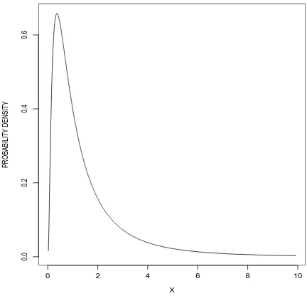
4.7
The exponential distribution
Suppose we have events occurring in a Poisson process of rate λ but we are in-terested in the random variable describing the time between events T. It can be shown that this random variable has an exponential distributionwith parameter
λ. The probability density function of an exponential random variable is given by:
f(t) =
λexp(−λt) for t >0.
0 otherwise, that is for t ≤0
This probability density function is shown with various values of λ in Fig-ure 7.
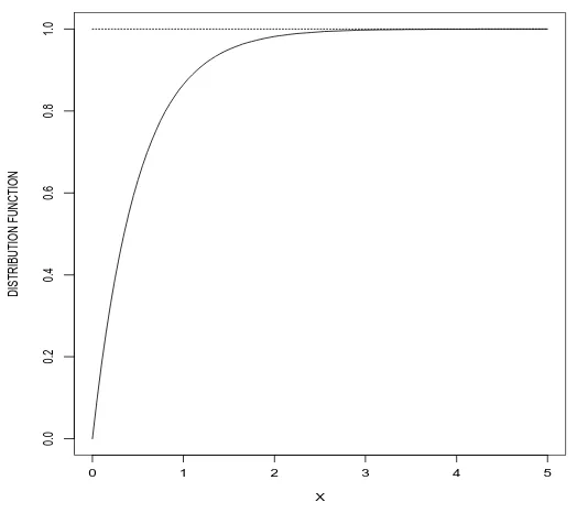
Notes: show that this is a probability density function and derive in lectures the distribution function, which is given by
X
PROBABILITY DENSITY FUNCTION
0 1 2 3 4 5
0.0 1.0 2.0 3.0
(a)
X
PROBABILITY DENSITY FUNCTION
0
1
2
3
4
0.0 1.0 2.0 3.0
(b)
X
PROBABILITY DENSITY FUNCTION
0 1 2 3 4 5
0.0 1.0 2.0 3.0
(c)
X
PROBABILITY DENSITY FUNCTION
0
1
2
3
4
0.0 1.0 2.0 3.0
X
DISTRIBUTION FUNCTION
0 1 2 3 4 5
0.0
0.2
0.4
0.6
0.8
1.0
As well as arising naturally as the time between events in a Poisson process the exponential distribution is also used to model the lifetimes of components which do not fail – the reason for this is the lack of memory property of the exponential distribution which will be discussed in lectures. This property states that:
P(T > s+t|T > s) = P(T > t).
4.8
The normal distribution
The normal distribution is of great importance for the following reasons: 1. It is often suitable as a probability model for measurements of weight, length, strength, etc.
2. Non-normal data can often be transformed to normality.
3. The central limit theorem states that when we take a sample of size n from any distribution with a mean µand a varianceσ2, the sample mean ¯X will have
a distribution which gets closer and closer to normality as n increases.
4. Can be used as an approximation to the binomial or the Poisson distributions when we have large n or λ respectively (though this is less useful now that computers can be used to evaluate binomial/Poisson probabilities).
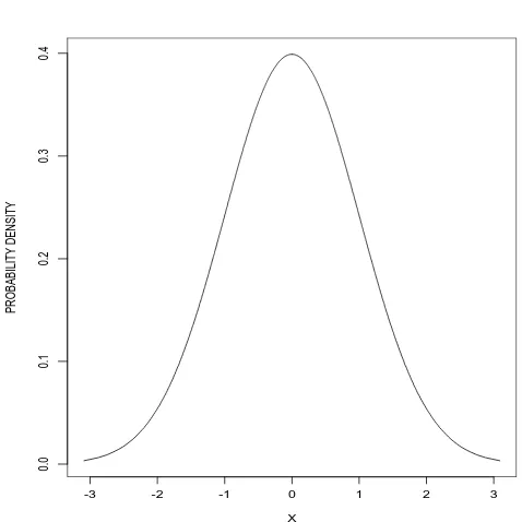
5. Many standard statistical techniques are based on the normal distribution. If the continuous random variable X has probability density function
φ(x) =f(x) = 1
(2π)1/2 exp
−x2/2− ∞< x <∞
We write X ∼N(0,1).
The standard normal distribution is symmetric about 0 and is shown in Figure 1.
The distribution function is given by:
F(x0) = P(X ≤x0) = Φ(x0) =
Z x0
−∞
1
(2π)1/2 exp
−x2/2dx.
This integral cannot be evaluated analytically hence its values are calculated numerically and are widely-tabulated. The density and distribution function of the standard normal distribution is shown in Figure 6.
Example 4.4: how to use standard normal tables.
4.9
Mean and variance
Recall in Section 1 we informally discussed measures of location and spread for sets of data. Here we define the mean and the variance as summaries of a distribution. Note that for some distributions the mean is not a good measure of the location of the distribution and the variance is not a good measure of the spread of a distribution. For normal data the mean and the standard deviation (which is the square root of the variance) are good summaries of location and spread.
For a discrete random variableX the expected value (or mean) is defined as
E(X) =
∞
X
i=1
xiP(X =xi).
For a continuous random variable with probability density functionf(x) the expected value (or mean) is defined as
E(X) =
Z ∞
−∞
Example 4.5: Properties:
(i) For constants a and b we have
E(aX +b) =aE(X) +b.
(ii) For random variables X and Y we have
E(X+Y) =E(X) +E(Y).
(iii) For constants a1, ..., ak and b and random variables X1, ..., Xk we have
E(a1X1+...+akXk+b) =a1E(X1) +...+akE(Xk) +b.
The variance of a random variable X is defined as
var(X) = E[(X−µ)2]
where
µ=E(X).
So the variance is the mean of the squared distances from the mean. The standard deviation is defined as
sd(X) = var(X)1/2.
Properties:
(i) For constants a and b we have
var(aX +b) =a2var(X).
(ii) For independent random variables X and Y we have
var(X+Y) = var(X) + var(Y).
(iii) For constantsa1, ..., ak and b and independent random variables X1, ..., Xk
we have
var(a1X1+...+akXk+b) =a21var(X1) + +...+a2kvar(Xk).
Examples:
Binomial distribution: E(X) = np, var(X) =np(1−p). Poisson distribution: E(X) = µ, var(X) =µ.
Uniform distribution: E(X) = (b+a)/2, var(X) = (b−a)2/12.
Exponential distribution: E(X) =λ−1
, var(X) = λ−2
.
Proofs: in class.
4.10
The normal distribution revisited
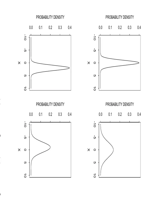
If the continuous random variable X has probability density function
f(x) = 1
σ(2π)1/2 exp −
(x−µ)2
2σ2
!
X PROBABILITY DENSITY -10 -5 0 5 10
0.0 0.1 0.2 0.3 0.4
X PROBABILITY DENSITY -10 -5 0 5 10
0.0 0.1 0.2 0.3 0.4
X PROBABILITY DENSITY -10 -5 0 5 10
0.0 0.1 0.2 0.3 0.4
X PROBABILITY DENSITY -10 -5 0 5 10
0.0 0.1 0.2 0.3 0.4
then X has a normal distribution with mean µ and standard deviation σ. We write X ∼N(µ, σ2). Figure 4 shows the effect of changing the values of µ and σ.
Important result: if X ∼N(µ, σ2) then the random variable Z defined by
Z = X−µ
σ
is distributed as Z ∼N(0,1). This is useful for looking up in tables the values of the distribution function for arbitrary normal distributions, that is, we don’t need a separate set of tables for each value of µ and σ.
Example 4.6: how to use the normal tables for arbitrary normal distributions. Further important results:
1. If X1 and X2 are independent random variables with distributionsN(µ1, σ2 1)
and N(µ2, σ2
2) respectively, then the random variable defined by
Z =X1+X2
is also normal with mean
E(Z) = E(X1) +E(X2) = µ1+µ2
and variance
var(Z) = var(X1+X2) = var(X1) + var(X2) = σ12+σ22.
2. If X1 and X2 are independent random variables with distributionsN(µ1, σ2 1)
and N(µ2, σ2
2) respectively, then the random variable defined by
is also normal with mean
E(Z) =E(X1)−E(X2) = µ1−µ2
and variance
var(Z) = var(X1−X2) = var(X1) + var(X2) =σ12+σ22.
3. General result If X1, ..., Xn are independent random variables with Xi ∼
N(µi, σ2i) and a1, ..., an are constants then the random variable defined by
Z =
n
X
i=1
aiXi
has a normal distribution with mean
E(Z) =E
n
X
i=1 aiXi
!
=
n
X
i=1 aiµi
and variance
var(Z) = var
n
X
i=1 aiXi
!
=
n
X
i=1 a2iσi2.
Very important result
Definition: a random sample of size n from a distribution f(x) is a set of independent and identically distributed random variables X1, ..., Xn each with
the distribution f(x).
If X1, ..., Xn are a random sample from the normal distribution N(µ, σ2)
then the random variable
¯
X = 1
n
n
X
i=1
Xi
E( ¯X) =µ
and variance
var( ¯X) = σ
2
n .
5
Statistical Analysis
5.1
Introduction
Probability theory provides us with models for random experiments. Such ex-periments provide realizations xof random variablesX. The observationX =x
is only one of many possible values of X. We wish to learn about the probabil-ity distribution or probabilprobabil-ity densprobabil-ity function which produced x – this will us allow us to make inference about the process under study.
For example, we will be able to predict future outcomes/summarize the under-lying system.
The notation we shall now use to represent our probability model is p(x|θ) where θ represents the parameter of the model – this notation makes explicit that to evaluate the probability of seeing a particular observation we need to know the value of θ.
In Section 4 the probability models which we looked at containedparameters, for example
(i) a binomial random variable with probability of success p so θ=p, (ii) a Poisson random variable with rate λ so θ=λ,
(iii) a normal random variable with mean µand variance σ2 soθ = (µ, σ2).
In Section 3 these parameters were assumed known and we could predict the outcomes we were likely to see, for example we could evaluate probabilities such as P(X >3).
After observing outcomes x1, x2, ...,xn we may be interested in:
Point estimation: guessing the value ofθ.
5.2
Point estimation
Suppose we obtain a random sample of size n from some probability model
f(x|θ). That is, we obtain measurements x= (x1, ..., xn) on n independent and
identically distributed random variables X = (X1, ..., Xn) each with the same
distribution f(x|θ).
In this case we have the joint distribution
f(x|θ) =f(x1, ..., xn|θ) = f(x1|θ)...f(xn|θ) = n
Y
i=1
f(xi|θ).
Viewing the joint distribution as a function of θ gives what is known as the
likelihood function.
Example: dataset 2, downloading times.
We could assume that x1, ...,x100 are a random sample from f(xi|µ, σ2) where
f(.|.) is a normal distribution, that is:
Xi ∼N(µ, σ2).
Definition: any real-valued function T = g(x1, ..., xn) of the observations in
the random sample is called a statistic.
T is known as an estimator if we use it as a guess of the value of some unknown parameter.
Example 5.1: A random sample of size 10 of response times were obtained (in seconds) for an online holiday booking query:
5.3, 4.9, 6.2, 5.7, 4.8
Suppose it were assumed that these measurements formed a random sample of size 10 from a normal distribution with mean µand known variance σ2 = 0.52.
How could we guess the value of µ?
Various possibilities are open to us: we could try the mean, the median, the average of the smallest and the largest ,...
How do we judge an estimator ?
Important idea: our estimatorT =g(X) is a function of the random variables
X1, ...,Xn and so the estimator itself has a distribution which is known as the
sampling distribution.
We would like the distribution of our estimator to be ‘close to the unknown parameter θ’ with high probability.
If we have a distribution for our estimator then how could we summarize this distribution?
(i) The average value: the estimator T =g(X) is said to be unbiased if
E[T] =θ
– on average we obtain the correct answer. If we repeated the experiment an infinite number of times then our average answer would be the correct answer. (ii) The variance: if we have two estimators that are unbiased then we would rather use the one which has the smaller variance.
Recall the result from Section 4 that if we have a random sample of size n
from the normal distribution N(µ, σ2) then
¯
X = 1
n
n
X
i=1
Xi
has a normal distribution with E[ ¯X] =µand var( ¯X) = σ2
So the sample mean is an unbiased estimator of µ. Example 5.1 revisited
Result: if we have a random sample of size n from the normal distribution
N(µ, σ2) with µ and σ2 both unknown then the estimator
T = 1
n−1
n
X
i=1
(Xi−X¯)2
5.3
Maximum Likelihood Estimation
One way of estimating the parameter θ, is by choosing the value of θ that maximises the likelihood:
L(θ) =
n
Y
i=1
f(xi|θ).
In other words, we choose θto give the highest probability to the observed data. This value of θ is known as the Maximum Likelihood Estimator (MLE). Example 5.2:
5.4
Interval estimation
We have seen that associated with any point estimator of an unknown parameter
θ there is a measure of the uncertainty of that estimator.
Example: Consider a random sample of size n X1, ..., Xn from N(µ, σ2) with
σ known but µunknown. The estimator ˆµ= ¯X has
E[ ¯X] =µ
and
var( ¯X) = σ
2
n .
An alternative method of describing the uncertainty associated with an esti-mate is to give an interval within which we think that θ lies. One way of doing this is via a confidence interval.
In lectures derive the confidence interval for the mean µ of a normal distri-bution when the varianceσ2 is known. The 100(1−α)% confidence interval is
¯
x− z√α/2σ
n ,x¯+ zα/2σ
√
n
!
where zα/2 is that value such that
1−α=P(−zα/2 < Z < zα/2)
where Z ∼ N(0,1). So for example for α = 0.10 we have z = 1.6449, for
α = 0.05 we have z = 1.9600 and for α = 0.01 we have z = 2.5758. These 3 cases are appropriate for confidence intervals of, respectively, 90 % , 95 % and 99 %.
Example 5.3:
Suppose now that X1, ..., Xn are a random sample from the normal
distri-bution N(µ, σ2) where now both µand σ2 are unknown.
In the case where σ2 was known we used the fact that
Z = ( ¯X−µ)
σ/√n
has the standard normal distribution N(0,1). We cannot do this here since σ
is unknown.
We can, however, replace σ by the estimator
s =
" n X
i=1
(Xi−X¯)2/(n−1)
#1/2
consider the new random variable
T = X¯ −µ
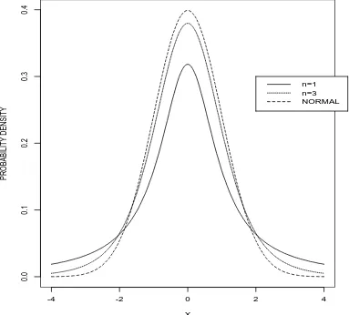
This random variable does not have a normal distribution but what is known as the (student’s) t-distribution with n − 1 degrees of freedom. The t-distribution is widely tabulated for different degrees of freedom. Like the normal distribution it is symmetrical about zero but has ‘fatter tails’, that is, there is more probability in the tails. As the degrees of freedom n tends to infinity the t-distribution tends to the normal distribution. The intuition here is that as we obtain more and more data our estimator for σ, namely s, becomes better and better in the sense that with high probability we will be close to the true value. Hence it is ‘as if’ we knew σand can use the normal distribution. Figure 1 shows a selection of t-distributions.
The confidence interval for µis given by:
¯
x− t√α/2s n ,x¯+
tα/2s
√n
!
where tα/2 is that value such that
1−α=P(−tα/2 < T < tα/2)
where T has a t-distribution with n−1 degrees of freedom.
Note: this interval is wider than when the variance σ2 is known, reflecting the
extra uncertainty in the estimate of σ2.
X
PROBABILITY DENSITY
-4 -2 0 2 4
0.0
0.1
0.2
0.3
0.4
n=1 n=3 NORMAL
6
Product Reliability
Let
T =
failure – time life – time
of a product e.g. an automobile, stereo, computing equipment.
The random variable, T is non-negative, by its nature and has distribution function F(t), the failure-time distribution, and probability density function
f(t), the failure-time density.
The probability that the product will fail before time t0:
P(T ≤t0) =F(t0) =
Z t0
0 f(t) dt.
The probability that the product will survive until time t0:
P(T > t0) = 1−F(t0) = R(t0), say.
R(t0) is the probability of reliability.
We note that,
f(t)dt≈P(t < T < t+ dt) = probability that a product will fail in (t, t+ dt).
6.1
Alternative ways to describe life characteristics of a
product
Let A be event ‘Product fails in (t, t+ dt)’
B be event ‘Product survives until t’
Probability of failure in (t, t+ dt), given survival until t, is
P(A|B) = P(A∩B) P(B) =
P(A) P(B) ≈
f(t) dt
1−F(t) =
f(t) dt R(t) . The quantity
z(t) = f(t)
R(t) ∝P(A|B) and is called the hazard rate of the product.
Knowledge about a product’s hazard rate often helps us to select the appro-priate failure time density function for the product.
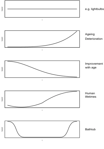
6.2
Examples of Hazards
Figure 11 shows some examples of hazard functions.
6.3
Examples of commonly used failure-time densities
6.3.1 Exponential Distribution
A positive random variable T has an exponential distribution with parameter
λ (λ >0) if its pdf is
f(t) =
λe−λt
t >0 0 otherwise.
The exponential distribution is used as the model for the failure time distribu-tion of systems under ‘chance’ failure condidistribu-tions, e.g.
2. Time intervals between successive breakdowns of an electronics system.
Figure 12 shows the reliability and hazard function for an exponential distribu-tion with λ= 1.
Example 6.1: Show
R(t) =e−λt
t >0
z(t) =λ t >0constant hazard rate.
6.3.2 Two parameter Weibull Distribution
A positive random variable T has a Weibull distribution with parameters λ, β
(λ, β >0) if its pdf is
f(t) =
λβ(λt)β−1
e−(λt)β
t≥0
0 t <0.
β is a shape parameter, λ is a scale parameter. Figure 13 shows the reliability and hazard functions for a Weibull distribution with λ= 1, and β = 0.5 and 3. Example 6.2:
Show
R(t) =e−(λt)β
t >0.
z(t) =λβ(λt)β−1
t >0not memoryless.
t
hazard e.g. lightbulbs
t
hazard
Ageing
Deterioration
t
hazard
Improvement with age
t
hazard
Human lifetimes
t
hazard Bathtub
t
0 1 2 3 4 5
0.0
0.2
0.4
0.6
0.8
1.0
λ =1
Reliability
t
0 1 2 3 4 5
0.8
0.9
1.0
1.1
1.2
λ =1
Hazard
t
0 1 2 3 4 5
0.2
0.4
0.6
0.8
1.0
λ =1, β =0.5
Reliability
t
0 1 2 3 4 5
0
2
4
6
λ =1, β =0.5
Hazard
t
0 1 2 3 4 5
0.0
0.2
0.4
0.6
0.8
1.0
λ =1, β =3
Reliability
t
0 1 2 3 4 5
0
20
40
60 λ =1, β =3
Hazard