SVM Example
Dan Ventura
April 16, 2009
Abstract
We try to give a helpful simple example that demonstrates a linear SVM and then extend the example to a simple non-linear case to illustrate the use of mapping functions and kernels.
1
Introduction
Many learning models make use of the idea that any learning problem can be made easy with the right set of features. The trick, of course, is discovering that “right set of features”, which in general is a very difficult thing to do. SVMs are another attempt at a model that does this. The idea behind SVMs is to make use of a (nonlinear) mapping function Φ that transforms data in input space to data in feature space in such a way as to render a problem linearly separable. The SVM then automatically discovers the optimal separating hyperplane (which, when mapped back into input space via Φ−1, can be a complex decision surface).
SVMs are rather interesting in that they enjoy both a sound theoretical basis as well as state-of-the-art success in real-world applications.
To illustrate the basic ideas, we will begin with a linear SVM (that is, a model that assumes the data is linearly separable). We will then expand the example to the nonlinear case to demonstrate the role of the mapping function Φ, and finally we will explain the idea of a kernel and how it allows SVMs to make use of high-dimensional feature spaces while remaining tractable.
2
Linear Example – when
Φ
is trivial
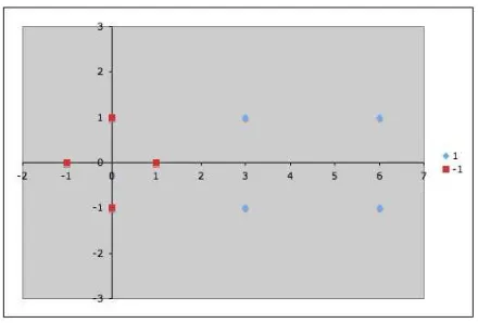
Suppose we are given the following positively labeled data points inℜ2
:
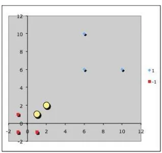
and the following negatively labeled data points inℜ2(see Figure 1):
Figure 1: Sample data points inℜ2. Blue diamonds are positive examples and
red squares are negative examples.
We would like to discover a simple SVM that accurately discriminates the two classes. Since the data is linearly separable, we can use a linear SVM (that is, one whose mapping function Φ() is the identity function). By inspection, it should be obvious that there are three support vectors (see Figure 2):
s1=
1 0
, s2=
3 1
, s3=
3
−1
In what follows we will use vectors augmented with a 1 as a bias input, and for clarity we will differentiate these with an over-tilde. So, ifs1 = (10), then
˜
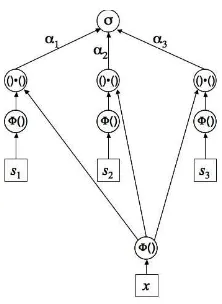
s1= (101). Figure 3 shows the SVM architecture, and our task is to find values
for theαi such that
α1Φ(s1)·Φ(s1) +α2Φ(s2)·Φ(s1) +α3Φ(s3)·Φ(s1) = −1
α1Φ(s1)·Φ(s2) +α2Φ(s2)·Φ(s2) +α3Φ(s3)·Φ(s2) = +1
α1Φ(s1)·Φ(s3) +α2Φ(s2)·Φ(s3) +α3Φ(s3)·Φ(s3) = +1
Since for now we have let Φ() =I, this reduces to
α1s˜1·s˜1+α2s˜2·s˜1+α3s˜3·s˜1 = −1
α1s˜1·s˜2+α2s˜2·s˜2+α3s˜3·s˜2 = +1
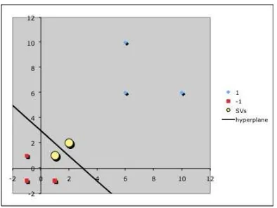
Figure 2: The three support vectors are marked as yellow circles.
2α1+ 4α2+ 4α3 = −1
4α1+ 11α2+ 9α3 = +1
4α1+ 9α2+ 11α3 = +1
A little algebra reveals that the solution to this system of equations isα1=
−3.5, α2= 0.75 andα3= 0.75.
Now, we can look at how theseαvalues relate to the discriminating hyper-plane; or, in other words, now that we have theαi, how do we find the
hyper-plane that discriminates the positive from the negative examples? It turns out that
Finally, remembering that our vectors are augmented with a bias, we can equate the last entry in ˜wwith the hyperplane offsetband write the separating hyperplane equation, 0 =wT
x+b, withw=
gives the set of 2-vectors withx1= 2, and plotting the line gives the expected
decision surface (see Figure 4).
2.1
Input space vs. Feature space
3
Nonlinear Example – when
Φ
is non-trivial
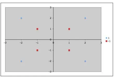
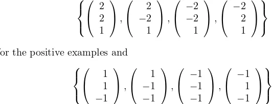
Now suppose instead that we are given the following positively labeled data points inℜ2:
and the following negatively labeled data points inℜ2
Figure 4: The discriminating hyperplane corresponding to the values α1 =
−3.5, α2= 0.75 andα3= 0.75.
Figure 5: Nonlinearly separable sample data points inℜ2. Blue diamonds are
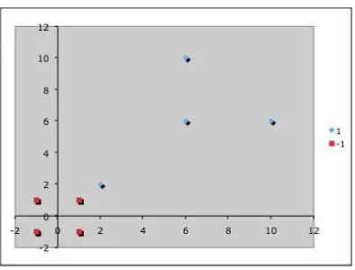
Figure 6: The data represented in feature space.
Our goal, again, is to discover a separating hyperplane that accurately dis-criminates the two classes. Of course, it is obvious that no such hyperplane exists in the input space (that is, in the space in which the original input data live). Therefore, we must use a nonlinear SVM (that is, one whose mapping function Φ is a nonlinear mapping from input space into some feature space). Define
Referring back to Figure 3, we can see how Φ transforms our data before the dot products are performed. Therefore, we can rewrite the data in feature space as
for the positive examples and
for the negative examples (see Figure 6). Now we can once again easily identify the support vectors (see Figure 7):
Figure 7: The two support vectors (in feature space) are marked as yellow circles.
α1Φ1(s1)·Φ1(s1) +α2Φ1(s2)·Φ1(s1) = −1
α1Φ1(s1)·Φ1(s2) +α2Φ1(s2)·Φ1(s2) = +1
Given Eq. 1, this reduces to
α1s˜1·s˜1+α2s˜2·s˜1 = −1
α1s˜1·s˜2+α2s˜2·s˜2 = +1
(Note that even though Φ1 is a nontrivial function, both s1 and s2 map to
themselves under Φ1. This will not be the case for other inputs as we will see
later.)
Now, computing the dot products results in
3α1+ 5α2 = −1
5α1+ 9α2 = +1
And the solution to this system of equations isα1=−7 andα2= 4.
Finally, we can again look at the discriminating hyperplane in input space that corresponds to theseα.
˜
w = X
i
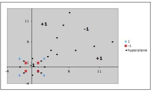
Figure 8: The discriminating hyperplane corresponding to the valuesα1 =−7
giving us the separating hyperplane equationy=wx+b withw=
1 1
and
b=−3. Plotting the line gives the expected decision surface (see Figure 8).
3.1
Using the SVM
Let’s briefly look at how we would use the SVM model to classify data. Given
x, the classificationf(x) is given by the equation
f(x) =σ X
i
αiΦ(si)·Φ(x)
!
(2)
whereσ(z) returns the sign ofz. For example, if we wanted to classify the point
Figure 9: The decision surface in input space corresponding to Φ1. Note the
singularity.
and thus we would classifyx= (4,5) as negative. Looking again at the input space, we might be tempted to think this is not a reasonable classification; how-ever, it is what our model says, and our model is consistent with all the training data. As always, there are no guarantees on generalization accuracy, and if we are not happy about our generalization, the likely culprit is our choice of Φ. Indeed, if we map our discriminating hyperplane (which lives in feature space) back into input space, we can see the effective decision surface of our model (see Figure 9). Of course, we may or may not be able to improve generalization accuracy by choosing a different Φ; however, there is another reason to revisit our choice of mapping function.
4
The Kernel Trick
Our definition of Φ in Eq. 1 preserved the number of dimensions. In other words, our input and feature spaces are the same size. However, it is often the case that in order to effectively separate the data, we must use a feature space that is of (sometimes very much) higher dimension than our input space. Let us now consider an alternative mapping function
Φ2
x1
x2
=
x1
x2
(x2 1+x22)−5
3
(3)
Figure 10: The decision surface in input space corresponding Φ2.
for the positive examples and
for the negative examples. With a little thought, we realize that in this case, all 8 of the examples will be support vectors withαi= 461 for the positive support
vectors and αi = −467 for the negative ones. Note that a consequence of this
mapping is that we do not need to use augmented vectors (though it wouldn’t hurt to do so) because the hyperplane in feature space goes through the origin,
y=wx+b, wherew=
andb= 0. Therefore, the discriminating feature,
isx3, and Eq. 2 reduces tof(x) =σ(x3).
Figure 10 shows the decision surface induced in the input space for this new mapping function.
Kernel trick.