ADAMA BAH
TNP2K WORKING PAPER 02 – 2013 October 2013
ESTIMATING VULNERABILITY TO
POVERTY USING PANEL DATA:
3
,
TNP2K Working Papers Series disseminates the findings of work in progress to encourage discussion and exchange of ideas on poverty, social protection and development issues. The publication of this series is supported by the
Government of Australia through the Poverty Reduction Support Facility (PRSF), for the Government of Indonesia’s National Team for Accelerating Poverty Reduction (TNP2K).
The findings, interpretations and conclusions herein are those of the author(s) and do not necessarily reflect the views of the Government of Australia or the Government of Indonesia.
The text and data in this publication may be reproduced as long as the source is cited. Reproductions for commercial purposes are forbidden.
Suggestion to cite: Bah, Adama (2013), ‘Estimating Vulnerability to Poverty Using Panel Data: Evidence from Indonesia’. TNP2K Working Paper 02-2013. Tim Nasional Percepatan Penanggulangan Kemiskinan (TNP2K): Jakarta, Indonesia.
To request copies of the paper or for more information on the series, please contact the TNP2K - Knowledge Management Unit ([email protected]).
Papers are also available on the TNP2K’s website (www.tnp2k.go.id)
TNP2K
Email: [email protected] :: [email protected] Tel: 021 391 2812
ADAMA BAH
TNP2K WORKING PAPER 02 – 2013 October 2013
ESTIMATING VULNERABILITY TO
POVERTY USING PANEL DATA:
4
ESTIMATING VULNERABILITY TO POVERTY USING PANEL DATA:
Evidence from Indonesia
Adama Bah
1October 2013
Abstract
Traditional poverty measures fail to indicate the degree of risk of becoming or remaining poor that households are confronted to. They can therefore be misleading in the context of implementing poverty reduction policies. In this paper I propose a method to estimate an index of ex ante
vulnerability to poverty, defined as the probability of being poor in the (near) future given current observable characteristics, using panel data. This method relies on the estimation of the expected mean and variance of future consumption conditional on current consumption and observable characteristics. It generates a vulnerability index, or predicted probability of future poverty, which performs well in predicting future poverty, including out of sample. About 80% of households with a 2000 vulnerability index of 100% are actually poor in 2007. This approach provides information on the population groups that have a high probability of becoming or remaining poor in the future, whether currently poor or not. It is therefore useful to complement traditional poverty measures such as the poverty headcount, in particular for the design and planning of poverty reduction policies.
Keywords: Poverty, Vulnerability, Household consumption.
JEL classification: C53, I32.
1 The National Team for the Acceleration of Poverty Reduction (TNP2K), Indonesia Vice-President Office, and CERDI-University of Auvergne, France – Email: [email protected]
5
Introduction
Poverty is inherently dynamic. Households that are poor at any point of time can be divided into two groups: those who have been poor for a certain period of time and those who have only recently fallen into poverty. Yet, traditional poverty measures such as the poverty headcount fail to account for this dynamic aspect of poverty, focusing on those who are currently poor regardless of their status in the past or in the future. While the poverty headcount provides valuable information, showing for instance that Indonesia has made considerable strides in reducing poverty in the past two decades,2 it misses part of the picture. Indeed, there is evidence of frequent movements in and out of poverty in Indonesia. For instance, it has been shown that over half of the poor each year are newly poor (World Bank, 2012). Using the Indonesian Family Life Survey (IFLS), a longitudinal survey conducted by the RAND Corporation, about 30% of households are found to have experienced poverty at least once between 1997, 2000 and 2007. This suggests that traditional poverty measures provide insufficient information and may be misleading in the context of the implementation of poverty reduction programs.
Reducing poverty is a top priority for the Government of Indonesia. In 2010, a National Team for the Acceleration of Poverty Reduction (Tim Nasional Percepatan Penanggulangan Kemiskinan, TNP2K) has been established under the leadership of the Vice-President. TNP2K has been mandated to coordinate and oversee the national poverty reduction strategy. This strategy is based on the premise that addressing poverty in an effective and sustainable manner requires reaching not only the current poor but also those at high risk of becoming poor in the near future. It comprises a range of social safety net programs covering education, health, food security, employment creation and community empowerment (see e.g. Sumarto and Bazzi 2011 for a review). Most of these programs originate from
6 the Asian Financial Crisis (AFC), which has had adverse effects on poverty in the country.3 These programs have the objectives to not only help the poor move out of poverty, but also to protect the vulnerable from falling into it. The vulnerable in this context are defined as households that are “just” above the poverty line, i.e. households living with 1.2, 1.4 or 1.5 times the national poverty line, depending on the program. In other words, for policy purposes it is considered that a household’s current consumption is the best predictor of its future consumption; households that are just above the poverty line are considered to be at a high risk of falling into poverty in the future.
In this paper, it is argued that at a given level of consumption, socioeconomic characteristics also matter for assessing the risk of becoming poor that households face. Indeed, household characteristics are likely to determine the degree of exposure to such risk, as well as their capacity to cope with it, for a given consumption level. I therefore propose a method to estimate vulnerability to poverty, defined as the probability of becoming poor in the future, given present observable characteristics. This method exploits the panel data available in the Indonesian Family Life Survey (IFLS). In particular, it relies on the estimation of the conditional distribution of future consumption to predict who is more likely to be below the poverty threshold in the future given their current characteristics, including consumption. It is found, for instance, that urban households with more children aged below 15 and with a member working as a private employee are more likely to experience a decrease in their future welfare, at a given consumption level. Larger households with an elderly head and self-employed members are on the other hand more subject to a higher variability in consumption.
The vulnerability estimates calculated using the panel-based method confirm that there is high vulnerability to poverty in Indonesia. In 2000, 60% of households were deemed vulnerable, having a vulnerability index, or probability of being poor in the future, greater than the poverty threshold. Furthermore, the panel-based vulnerability measures provide accurate predictions of future poverty, including in a context of steadily decreasing poverty rates. I find that an out-of-sample vulnerability
7 index constructed for 2000 provides good predictions of actual poverty realizations in 2007. About 80% of households with a 2000 vulnerability index of 100% are actually poor in 2007.
The remainder of the paper is organized as follows. Section 2 describes the Indonesian Family Life Survey used for the analysis. Section 3 provides a descriptive analysis of poverty in Indonesia and its dynamics. Section 4 introduces the panel-based method used to estimate vulnerability to poverty. Section 5 discusses the results, and section 6 provides concluding remarks.
Section 2 – The Indonesian Family Life Survey
The Indonesian Family Life Survey (IFLS)4 used in this paper to analyze poverty and vulnerability is an ongoing longitudinal survey conducted by the RAND Corporation. Its first round, IFLS1, was implemented in 1993 using the sampling frame of the 1993 national socioeconomic survey, the SUSENAS,5 in which the population was stratified first by provinces and then by (urban/rural) areas within the provinces. The IFLS1 sample was representative of 83% of the Indonesian population from 13 provinces.6 It surveyed 7,224 households and more than 22,000 individuals. The subsequent waves of the IFLS were implemented in 1997, 2000 and 2007, and re-surveyed original IFLS1 households. In this paper, the IFLS1 is not used since questions for non-food expenditures have been changed in the subsequent waves, making consumption not comparable with the one from the IFLS1 (Strauss et al. 2009).
The IFLS collects information on a wide array of household and individual characteristics, including demographic characteristics, household economy and expenditures, asset holdings, and education and health indicators. Yet, its most relevant feature for the purpose of this paper is the particular attention given to tracking IFLS1 households in the subsequent waves, including those that moved, in order to minimize attrition in the survey. As a result, the attrition rate in the IFLS is relatively low compared to
4 For more information on the IFLS go to: http://www.rand.org/labor/FLS/IFLS.html
5 The SUSENAS is a nationally representative socioeconomic survey conducted by the Indonesian National Statistics Office (Badan Pusat
Statistik, BPS).
8 similar surveys conducted in developing countries: 6,624 households, or 88% of the original sample, have been surveyed in all the three waves considered in this paper. The IFLS is also designed to track and survey individuals who split off from the original IFLS1 households to form new households,7 which increased the sample size in each consecutive wave.8
Estimating poverty dynamics and vulnerability to poverty requires the definition of a poverty threshold (poverty line). Provincial urban/rural poverty lines are available for the 2000 IFLS wave, from Strauss et al. (2004). These lines are the February 1999 poverty lines calculated by Pradhan et al. (2001) and inflated to represent 2000 prices following Suryahadi et al. (2003).9 I deflate and inflate these 2000 IFLS lines to obtain poverty lines for 1997 and 2007 respectively. Poverty lines for 1997 are obtained by deflating the 2000 lines using the re-weighted Consumer Price Index, following Suryahadi et al. (2003). For 2007, I inflate the 2000 IFLS lines using the inflation rate of the provincial urban/rural poverty lines between 2000 and 2007.10,11
Section 3 – A descriptive analysis of poverty dynamics
3.1 Changes in the poverty headcount over time
In this section, I first look at the changes in poverty over time using the cross-section data sets from each IFLS wave. I then focus on households that have been surveyed in all three waves (panel households).
7 See Witoelar (2005) for details on the tracking rules and their implications.
8 The 1997, 2000 and 2007 cross-sectional datasets have respectively a sample size of 7,087; 10,257 and 12,945 households. 9
The Consumer Price Index (CPI) is the weighted sum of the change in prices for food and non-food categories. Normally, food items represent 40% of the value of CPI. Suryahadi et al. (2003) changed the CPI weights to have food represent 80% of its value, since the share of food expenditures in the poverty lines in 1996 is also 80%. This change reflects that the poor are relatively more affected by changes in food prices than by changes in non-food prices. Another reason for re-weighing the CPI is that it is calculated only for urban areas. 10 For 2007, I do not use the re-weighted CPI because in 2003, the National Statistic Office (BPS) changed the base year for the CPI. The CPI in 2000 is thus not directly comparable with the 2007 one. In addition, between 2000 and 2007, the number of cities whose price levels are used for the CPI calculation has increased to 66 cities.
9
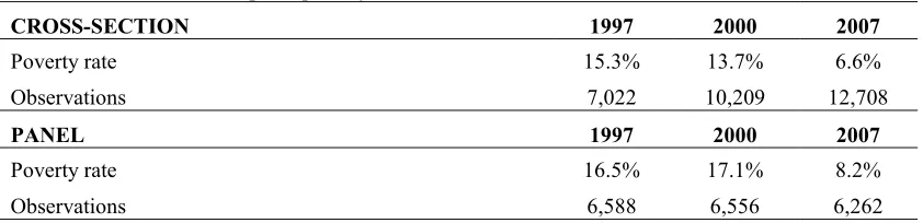
Table 1. Cross-section and panel poverty estimations
CROSS-SECTION 1997 2000 2007
Poverty rate 15.3% 13.7% 6.6%
Observations 7,022 10,209 12,708
PANEL 1997 2000 2007
Poverty rate 16.5% 17.1% 8.2%
Observations 6,588 6,556 6,262
Note: cross-section estimates use cross-sectional weights and (balanced) panel estimates use longitudinal weights corrected for attrition (Strauss et al. 2009), here and in the subsequent tables.
Table 1 shows that absolute poverty in the IFLS sample has decreased over time for both cross-sectional and panel households, which is in line with the trend recorded by the national poverty rates. Among the panel households (surveyed in all three waves), the poverty headcount increases slightly from 1997 to 2000 and is overall higher.
The differences between the cross-section and panel data poverty estimates are likely to be caused by two factors: the split-off effect and attrition. Poverty rates are lower in the cross-section because the split-off households are added in each cross-section. It is indeed likely that split-off households are better off than the original households in terms of per capita consumption. The second phenomenon affecting the poverty estimates is attrition. In developing countries, attrition occurs largely because households change their location, rather than due to their refusal to participate in the survey. In the IFLS however, attrition is lower than in similar longitudinal surveys because of the effort made to follow households that have moved, even to other provinces.12 According to Thomas et al. (2001), the per capita expenditure increases between 1993 and 1997 are more than 75% higher for households that moved compared to those that did not. Therefore, poverty estimates would be overestimated if households that moved since the last wave of the survey had not been interviewed in subsequent waves. Yet, it does not solve everything. As shown by Thomas et al. (2012), respondents who are most likely to drop out from the survey (and cannot be tracked) are better off in terms of education, health, parents’ and household characteristics.
10
3.2 Poverty dynamics
The panel data provides a more complete picture of poverty and socioeconomic mobility. It allows establishing whether a household is poor or not at a certain point of time, as well as assessing the changes in its status from one period to the other. Households that are below the poverty line in all 3 waves of the survey are defined as chronic poor; those who have been below the poverty line only in one or two periods are defined as transient poor.13
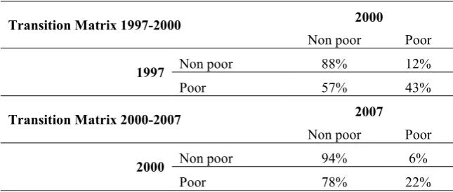
Table 2 shows the poverty transition matrices, which capture movements in and out of poverty. Overall, these results indicate significant socioeconomic mobility,14 with frequents movements in and out of poverty, for both poor and non-poor households. The decrease in poverty over time is observed with the decrease in the share of non-poor that become poor between 2000 and 2007 compared to between 1997 and 2000. It is also seen with the decrease in the share of poor households that remain poor between 2000 and 2007. Current poverty remains however a relatively good predictor of future poverty.
Table 2. Poverty dynamics among panel households 1997-2000-2007
Transition Matrix 1997-2000 2000
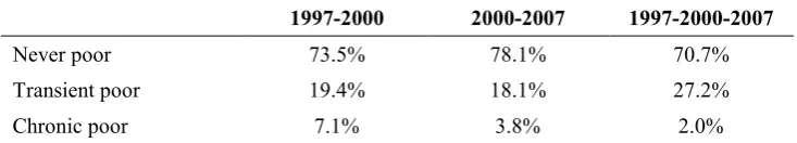
Table 3 summarizes the changes in households’ socioeconomic status over the entire period covered by the panel data. From 1997 to 2007, 29% of the sampled households are found poor in at least one wave, and the overwhelming majority of them are transient poor, having been poor in one or two waves. This large percentage of transient poor households provides evidence of high levels of
13 It is recognized that there is a 7-year gap between waves 3 and 4, thus it is a restrictive definition of chronic poverty. Further, some of the chronic poor might have been non-poor and some point during that gap, generating possible underestimation and overestimation of chronic poverty (similarly with those never poor).
11 vulnerability to poverty in Indonesia. It suggests that households are highly exposed to risks and are not adequately equipped to maintain their welfare levels in face of such risks.
Note that the share of households that are chronically poor decreases between the period 1997-2000 and the next, and only 2% of households are poor in all 3 waves. From a policy perspective, this suggests that this group increasingly marginalized may be potentially difficult to reach through traditional poverty reduction policies and programs.
Table 3. Type of poverty 1997-2007
1997-2000 2000-2007 1997-2000-2007
Never poor 73.5% 78.1% 70.7%
Transient poor 19.4% 18.1% 27.2%
Chronic poor 7.1% 3.8% 2.0%
Note: Transient poor are those that have been below the poverty line only in one or two periods; chronic poor are those that are below the poverty line in all the waves considered.
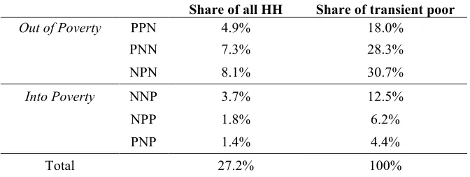
Table 4 disaggregates the information presented in Table 3 in order to get a better sense of the specific paths experienced by the transient poor in the three waves. In line with the decreasing poverty headcount rates, the large majority of transient poor have been moving out of poverty. However, 23% went from non-poor to poor over the period 1997-2007. Household vulnerability to falling into poverty therefore appears to remain an issue even in a context where overall poverty headcount rates are decreasing. This can be further seen with the relatively large share of households that do not have the same poverty status in two consecutive waves (NPN and PNP), which amount to 35% of the transient poor.
12
Table 4. Pathways of the transient poor over 1997-2000-2007.
Share of all HH Share of transient poor
Note: HH=households. P=Poor; N=Not poor; this represents the poverty status in each IFLS wave.
Section 4 – Measuring vulnerability to poverty: an analytical framework
The previous section has shown that poverty in Indonesia is for the most part a transient phenomenon. This highlights the limitations of traditional poverty measures, which present households which are above or below the poverty line at a certain point in time as homogeneous groups. They fail to account for the fact that within these two groups some households are exposed to numerous risks that they might not be able to mitigate and that can therefore worsen their living conditions. Vulnerability is an important aspect of poverty analysis that allows introducing a dynamic dimension to poverty assessments.
There are different definitions and approaches to measuring vulnerability in the literature (see Hoddinott and Quisumbing (2003) and Ligon and Schechter (2004) for an overview). In general, vulnerability is a forward looking concept. I use a practical definition of vulnerability, as the risk (or probability) that a household will be poor in the future, given what can be observed of its characteristics now. These observable characteristics include current (per capita) consumption as well as a broad set of (socioeconomic) indicators. Vulnerability can thus be expressed as follows:
𝑉𝑢𝑙𝑖𝑡 =𝑃( 𝑝𝑜𝑜𝑟𝑖𝑡+1= 1 | 𝑋𝑖𝑡,𝑃𝐶𝐸𝑖𝑡) (4.1)
13 vulnerable to being poor in the future are those that have a low expected welfare level and/or are subject to a high variability in that welfare. I model here the expected mean and variance of households’ future per capita consumption.
The conditional mean of the log of future consumption expenditures is assumed linear in the log of current consumption and household characteristics. The regression form is given by:
ln𝑃𝐶𝐸𝑖𝑡+1 =𝛼+𝛽𝑋𝑖𝑡 +𝛾ln𝑃𝐶𝐸𝑖𝑡+𝜀𝑖𝑡+1 (4.2)
Where 𝑃𝐶𝐸𝑖𝑡+1 and 𝑃𝐶𝐸𝑖𝑡 are household future and current per capita expenditures respectively, 𝑋𝑖𝑡 is a vector of household socioeconomic characteristics. I assume that the error term is conditionally mean independent of 𝑃𝐶𝐸𝑖𝑡 and 𝑋𝑖𝑡, i.e.𝐸[𝜀𝑖𝑡+1| ln𝑃𝐶𝐸𝑖𝑡,𝑋𝑖𝑡] = 0.
Similar to Chaudhuri et al. (2002), I also model the conditional variance of future per capita expenditures. The conditional variance is assumed linear in the log of current per capita expenditures
and household characteristics. Given that
𝐸[(ln𝑃𝐶𝐸𝑖𝑡+1− 𝐸[ln𝑃𝐶𝐸𝑖𝑡+1| ln𝑃𝐶𝐸𝑖𝑡 ,𝑋𝑖𝑡])2| ln𝑃𝐶𝐸𝑖𝑡 ,𝑋𝑖𝑡] =𝐸�𝜀𝑖𝑡+12 | ln𝑃𝐶𝐸𝑖𝑡 ,𝑋𝑖𝑡�, the
regression model of the variance is written as follows:
(𝜀𝑖𝑡+1)2=𝛼�+𝛽�𝑋𝑖𝑡+𝛾�ln𝑃𝐶𝐸𝑖𝑡 + 𝑢𝑖𝑡+1 (4.3)
This two equation model is estimated sequentially using Ordinary Least Squares (OLS). In the first step, I estimate (4.2), and the parameter estimates obtained are used to construct the residuals 𝜀̂𝑖𝑡+1. The squared residuals parameters are then used in (4.3) to estimate the conditional variance of household future per capita expenditures.
14 Chaudhuri et al. (2002) approach.15 In the empirical section I conclude that their procedure is rather weak in terms of accurately predicting future poverty.
One way in which the approach developed here differs from Chaudhuri et al. (2002) is by the inclusion of current consumption as one of the predictors of future consumption. This allows accounting for threshold effects that would be associated with poverty traps, among others. Indeed, current expenditure levels are the best predictors for future expenditure levels. In addition, the approach adopted here also allows estimating whether, at a given level of current welfare, different households are more subject to shocks (and/or have different access to and use of coping mechanisms) than others.16
Following Chaudhuri et al. (2002), I assume that future consumption is log-normally distributed, with the estimated conditional mean and variance obtained through the two-step regression approach above. This allows estimating household vulnerability to poverty - or the probability of being poor in the future – conditional on current consumption and household characteristics, by:
𝑉𝑢𝑙�𝑖𝑡=𝑃𝑟�(ln𝑃𝐶𝐸𝑖𝑡+1< ln𝑝𝑙| 𝑃𝐶𝐸𝑖𝑡,𝑋𝑖𝑡) =Φ �ln 𝑝𝑙−𝐸��𝑉�[ln 𝑃𝐶𝐸[ln 𝑃𝐶𝐸𝑖𝑡+1| 𝑃𝐶𝐸𝑖𝑡,𝑋𝑖𝑡]
𝑖𝑡+1| 𝑃𝐶𝐸𝑖𝑡,𝑋𝑖𝑡] � (4.4)
Where pl is the poverty line.
Another way to estimate (4.1) is to directly estimate the probability of being poor in t+1 using a probit model, thereby making the assumption that the conditional variance of future per capita expenditures is constant across households. This model is simpler to implement, and therefore provides an interesting comparison. It allows, for instance, assessing the importance of allowing the inter-temporal variance in consumption to depend on household current consumption and characteristics.
15 See Chaudhuri (2002) and Chaudhuri, Jalan and Suryahadi (2002) for details on the method.
15
Section 5 – Results
5.1 Vulnerability estimates
I estimate the panel data models introduced in the previous section using the 1997 and 2000 waves of the IFLS.17 The cross-sectional model described in Chaudhuri et. al. (2002) is estimated for 1997 and 2000. The 2007 wave of the IFLS is used to evaluate the respective performances of these models, out of sample, in the next section. In all regressions, a set of characteristics representing household demographics, educational attainment, labor market participation, access to basic (energy) services, assets and social capital are used. Most are derived from the correlates identified as best predictors of welfare using the approach developed in Bah (2013).18
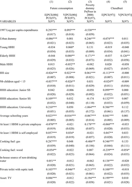
The results of the vulnerability regressions using the 2 methods described in the previous section are displayed in Table 5. Columns (1) and (2) of Table 5 show the results of the estimation of the expected mean and variance of the future consumption distribution, which we will refer to below as
consumption-based, and columns (3) shows the probit regressions results, which we will refer as
poverty dummy-based. Columns (4) and (5) display the results from the Chaudhuri method relying on cross-section, for comparison.
Table 5 shows that the 1997 consumption level is significantly associated with future consumption and poverty. The consumption- and poverty dummy-based estimates generate similar results in terms of the variables associated with future poverty. The parameters have opposite signs, since being poor implies having a lower expected consumption.
Urban households, interestingly, as well as large households with more children aged below 15 and those with at least a member working as a private employee, appear more likely to have a lower future welfare level and be poor at a given level of (current) welfare. Households with a higher educational
17 Note that all per capita expenditures are appropriately deflated to capture regional price variation and to represent constant levels of welfare over time.
16 attainment (both of the head and on average in the household), with in-house access to non-drinking water, with a private toilet with septic tank and households cooking with gas are significantly less likely to becoming poor in the future, at a given welfare level. Interestingly, households that have accumulated assets appear better able to deal with adverse shocks at the same consumption level.
In addition, it appears that the conditional variance of future consumption also varies significantly across household characteristics. Larger households with an elderly head are likely to have a higher variability in consumption, which also translates into having a higher probability of becoming poor at a given level of consumption. Household size is thus a variable that is not only associated with lower expected future welfare, but also with more risk to that welfare, whereas household average schooling years and disposing of private toilet with septic tank are both associated with a higher and less risky future welfare. Households with at least one self-employed member appear to have both a higher expected future welfare and higher variability in that welfare. It is also interesting to note that participating in arisan19 is associated with a higher future expected welfare level, but not with the variability in that welfare. This suggests that these community- or network-level saving groups might not be efficient in insuring households against consumption fluctuations.
The future consumption-based estimates (columns 1-2) are in a sense similar to the results of the Chaudhuri approach (columns 4-5). The main difference lies in the fact that in column 1-2 current consumption is included as a predictor of future consumption. Current consumption appears clearly the best predictor of future consumption (with a t statistic of about 30).
17
1997 Log per capita expenditures 0.293*** 0.095*** -0.530*** (0.017) (0.018) (0.059) HHH education: University 0.210*** 0.050 -1.064*** 0.386*** 0.112
18
Notes: HH stands for household, HHH for household head and HHM for household member. Arisan is a rotating savings group. For the Probit regression (column 3), R-squared is the MacFadden Pseudo-R-squared. Standard errors in parentheses. *** p<0.01, ** p<0.05, * p<0.1
5.2 Assessing the predictive power of vulnerability estimates for future poverty
The use of panel data to estimate vulnerability has been relatively neglected in the literature because of the relative scarcity of panel surveys in developing countries. However, I show in this section that estimating vulnerability using panel data provides significantly better predictions of future poverty (in and out of sample), and should therefore be preferred.20
Data from a two-wave panel can be used to estimate parameters. The parameters can be applied to compute vulnerability indexes in alternative (potentially cross-sectional) data sets, like the SUSENAS (for the Indonesian case). Newer rounds of panel data can then be used to update the parameters needed for computing vulnerability indexes. To prove this point, I provide an out-of-sample comparison of the predictions of the panel-based vulnerability measures with the ones from the Chaudhuri et al. (2002) method. Using the parameter estimates from table 5, I construct consumption- and poverty dummy-based vulnerability indexes for 2000. I then compare the predictions of these measures and the Chaudhuri measures for 1997 and 2000 to actual poverty realizations in 2007.
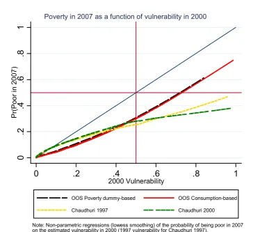
19 The relationship between the vulnerability indexes in 2000 and actual poverty in 2007 are presented in Figure 1. I find that all vulnerability measures underestimate the real likelihood of being poor in 2007 - they are all below the 45-degree line. The consumption- and poverty dummy-based measures however appear to be significantly better predictors of future poverty compared to the (1997 and 2000) Chaudhuri measures. The better predictive power of the out-of-sample (OOS) panel-based measures is most apparent in the top-right area (which is the most relevant area) of the graph, the area where households have a vulnerability index of 50% and above. The panel data methods are much closer to what actually happened in 2007. For example, nearly 80% of the households with a vulnerability index of 100% were actually poor in 2007 (wrongly predicting only 20% of these observations). In contrast, less than 40% of households deemed future poor with a high probability – vulnerability index above 50% - by the Chaudhuri measures actually became poor in 2007. In other words, the cross sectional method has severe difficulties identifying the highly vulnerable.
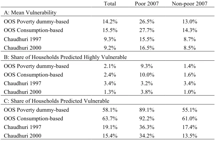
Table 6 shows the same vulnerability estimates, disaggregated for the 2007 poor and non-poor. Panel A shows the mean of the 2000 vulnerability estimates (consumption- and poverty dummy-based are out-of-sample estimates), or predicted future poverty rates; panel B shows the share of households predicted highly vulnerable - vulnerability index greater than 50% - and panel C shows the share of households predicted vulnerable - vulnerability index greater than the current poverty rate.
20
Figure 1 - Cross-validation of the Vulnerability Measures
Among the poor, the consumption- and dummy-based estimates appear higher than the Chaudhuri measures. In particular, for the share of households predicted highly vulnerable, the Chaudhuri 1997 measure does not allow distinguishing between the poor and non-poor in 2007. About 3% of both poor and non-poor have a Chauduri 1997 vulnerability index above 50%, compared to 9-10% of the 2007 poor that are predicted highly vulnerable by the panel-based measures. . Among the poor households of 2007, about 90% are predicted vulnerable according to the out-of-sample consumption- and poverty dummy-based vulnerability measures, compared to about 35% for the Chaudhuri measures. This out-of-sample exercise thus validates the high predictive power of the consumption- and poverty dummy-based measures for future poverty.
0
Note: Non-parametric regressions (lowess smoothing) of the probability of being poor in 2007 on the estimated vulnerability in 2000 (1997 vulnerability for Chaudhuri 1997).
Probit and consumption-based vulnerability measures are out-of-sample estimates, i.e. constructed by applying parameters estimated on 1997 data to 2000 data.
21
Table 6: 2000 vulnerability estimates and 2007 actual poverty
Total Poor 2007 Non-poor 2007 A: Mean Vulnerability
OOS Poverty dummy-based 14.2% 26.5% 13.0% OOS Consumption-based 15.5% 27.7% 14.3%
Chaudhuri 1997 9.3% 15.5% 8.7%
Chaudhuri 2000 9.2% 16.5% 8.5%
B: Share of Households Predicted Highly Vulnerable
OOS Poverty dummy-based 2.1% 9.3% 1.4% OOS Consumption-based 63.7% 92.2% 61.0% Chaudhuri 1997 19.1% 36.3% 17.4% Chaudhuri 2000 15.4% 34.2% 13.5%
Notes: OOS stands for out-of-sample, i.e. obtained from applying parameters estimated using (consumption and household characteristics) 1997 data to (consumption and household characteristics) data from 2000. Households predicted highly vulnerable are those with a vulnerability index above 50%; households predicted vulnerable are those with a vulnerability index above the 2000 poverty rate (17.1% - see table 1).
Section 6 – Concluding remarks
In this paper, it is confirmed that, although Indonesia has been quite successful in decreasing the poverty rate over the past decades, there has been a large socioeconomic mobility over 1997, 2000 and 2007, with frequent movements in and out of poverty. A large proportion of the population (27%) has experienced poverty at least once.
22 of future poverty: about 80% of the households with a 2000 vulnerability index of 100% were actually poor in 2007. The accuracy of these out-of-sample vulnerability estimates provides a good argument for implementing the method using one (panel) sample and applying the parameters obtained in another (potentially cross-sectional) sample in order to predict the probability of future poverty.
In Indonesia, as mentioned earlier, vulnerability is currently defined as the population that lives with up to 1.2 or 1.4 times the poverty line. This definition has been used recently for determining the coverage of the Social Protection Card (Kartu Perlindungan Sosial – KPS) launched in June 2013. Using this card, eligible households are entitled to receiving benefits from three social protection programs – a rice subsidy program, (Beras untuk Rumah Tangga Miskin – Raskin); a scholarship program (Bantuan Siswa Miskin – BSM); and a temporary unconditional cash transfer program
(Bantuan Langsung Sementara Masyarakat - BLSM). The KPS currently covers 15.5 million
households, which corresponds to the poorest 25% of the Indonesian population.
The method proposed in this paper confirms that current consumption is an important predictor of future consumption – and its variability. Furthermore, at a given level of consumption, certain household characteristics such as the average schooling level or the working status of the head are associated with higher vulnerability to poverty. Using this method in combination with the reference to the poverty line currently applied in Indonesia would therefore allow fine-tuning the definition of the target for social protection programs – i.e. vulnerable households.
24
References
Bah, A. (2013): “Finding the Best Indicators to Identify the Poor”, TNP2K Working Paper 01-2013, The National Team for the Acceleration of Poverty Reduction (TNP2K): Jakarta, Indonesia.
Baulch, B., & Hoddinott, J. (2000): “Economic mobility and poverty dynamics in developing countries”. The Journal of Development Studies, 36(6), 1-24.
Chaudhuri, S. (2000): “Empirical Methods for Assessing Household Vulnerability to Poverty”, mimeo, Department of Economics, Columbia University: New York.
Chaudhuri, S., Jalan, J. and A. Suryahadi (2002): “Assessing household vulnerability to poverty from cross-sectional data: A methodology and estimates from Indonesia”, Department of Economics Columbia University. Available at: http://digitalcommons.libraries.columbia.edu/econ dp/117.
Chaudhuri, S. (2003): “Assessing vulnerability to poverty: concepts, empirical methods and illustrative examples”, Department of Economics Columbia University. Available at:
http://info.worldbank.org/etools/docs/library/97185/Keny_0304/Ke_0304/vulnerability-assessment.pdf.
Dercon, S., and P. Krishnan (2000): “Vulnerability, seasonality and poverty in Ethiopia”, The Journal of Development Studies, 36(6), 25-53.
Hoddinott, J. and A. Quisumbing (2003): “Methods for Microeconometric Risk and Vulnerability Assessments”, Social Protection Discussion Paper Series No. 0324, The World Bank, Washington D.C.
Kochar, A. (1995): “Explaining household vulnerability to idiosyncratic income shocks”. The American Economic Review, 85(2), 159-164.
Ligon, E. and L. Schechter (2003): “Evaluating Different Approaches to Estimating Vulnerability”, Social Protection Discussion Paper Series, No.0410. Social Protection Unit, Human Development Network, The World Bank, Washington D.C.
Maksum, C. (2004): “Official Poverty Measurement in Indonesia”, Paper presented at the International Conference on Poverty Statistics, 4-6 October 2004, Mandaluyong City, Philippines. Pradhan, M., A. Suryahadi, S. Sumarto, and L. Pritchett (2003): “Eating Like Which “Joneses?” An Iterative Solution to the Choice of a Poverty Line “Reference Group””. Review of Income and Wealth
47 (4): 473–487.
Pritchett, L., Suryahadi, A., and S. Sumarto (2000): “Quantifying vulnerability to poverty, A proposed measured applied to Indonesia” Policy Research Working Paper No. 2437, The World Bank East Asia and Pacific Region, Environment and Social Development Sector Unit.
Ravallion, M., and M. Lokshin (2007): “Lasting Impacts of Indonesia’s Financial Crisis”, Economic Development and Cultural Change, 56 (1): 27-56
Strauss, J., K. Beegle, B. Sikoki, A. Dwiyanto, Y. Herawati and F. Witoelar (2004): “The Third Wave of the Indonesia Family Life Survey (IFLS3): Overview and Field Report”, RAND Labor and Population, March 2004. WR-144/1-NIA/NICHD.
25 Sumarto, S. and S. Bazzi (2011): “Social Protection in Indonesia: Past Experiences and Lessons for the Future”, Paper presented at the 2011 Annual Bank Conference on Development Opportunities (ABCDE) jointly organized by the World Bank and OECD, 30 May-1 June 2011, Paris.
Suryahadi, A. and S. Sumarto (2003): “Poverty and Vulnerability in Indonesia Before and After the Economic Crisis” Asian Economic Journal 17 (1): 45-64.
Suryahadi, A., S. Sumarto , and L. Pritchett (2003): ‘Evolution of Poverty During the Crisis in Indonesia.’ Asian Economic Journal 17 (3): 221–241.
Thomas, D., Frankenberg, E. and J.P. Smith (2001): “Lost but Not Forgotten: Attrition and Follow-up in the Indonesia Family Life Survey”. Journal of Human Resources, 36, 556-592.
Thomas, D., Witoelar, F., Frankenberg, E., Sikoki, B., Strauss, J., Sumantri, C., and W. Suriastini (2012): “Cutting the costs of attrition: Results from the Indonesia Family Life Survey”, Journal of Development Economics, 98(1), 108-123.
Widyanti, W., Sumarto, S. and A. Suryahadi (2001): “Short-term Poverty Dynamics: Evidence from Rural Indonesia”, SMERU Research Institute Working Paper: Jakarta, Indonesia.
Widyanti, W., Suryahadi, A., Sumarto, S. and A. Yumma (2009): “The Relationship between Chronic Poverty and Household Dynamics: Evidence from Indonesia” SMERU Research Institute Working Paper: Jakarta, Indonesia.
26
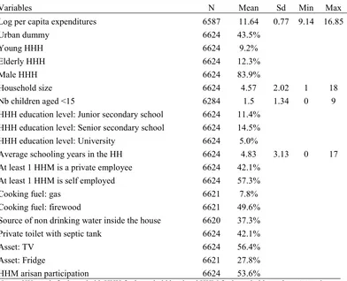
Table A1: List of explanatory variables from 1997 and their descriptive statistics
Variables N Mean Sd Min Max
Log per capita expenditures 6587 11.64 0.77 9.14 16.85
Urban dummy 6624 43.5%
Young HHH 6624 9.2%
Elderly HHH 6624 12.3%
Male HHH 6624 83.9%
Household size 6624 4.57 2.02 1 18
Nb children aged <15 6284 1.5 1.34 0 9 HHH education level: Junior secondary school 6624 11.4%
HHH education level: Senior secondary school 6624 14.5% HHH education level: University 6624 5.0%
Average schooling years in the HH 6624 4.83 3.13 0 17 At least 1 HHM is a private employee 6624 42.1%
At least 1 HHM is self employed 6624 57.3%
Cooking fuel: gas 6621 7.8%
Cooking fuel: firewood 6621 49.6% Source of non drinking water inside the house 6620 37.3% Private toilet with septic tank 6624 42.1%
Asset: TV 6624 56.4%
Asset: Fridge 6621 27.8%
HHM arisan participation 6624 53.6%